3 SFC model presentation

Flexible rate mortgage loans: An SFC model of the impact of mortgage credit innovations on Danish balance sheet stability

Abstract

Innovations in mortgage lending options have expounded in recent decades, resulting primarily in a reduction in the initial monthly costs associated with borrowing, and made home ownership possible for socio-economic groups that were previously excluded from the market. These changes have also drastically changed the composition of household balance sheets, both at a micro and a macro level, and the volume of outstanding debt relative to household income expanded aggressively leading up to the global financial crisis in 2007-8. The innovations unfortunately also simultaneously transferred significant risks to borrowers. This paper investigates the present day macroeconomic consequences of the change in composition from fixed- to adjustable-rate mortgage (ARM) debt that occurred in Denmark between 2003 and 2009. A state-of-the-art Stock-Flow Consistent model is adapted to allow for changes in the composition of debt, and to permit shifts in the proportion of debt between fixed-interest and ARM products. The risks to financial stability are evaluated through the imposition of two plausible shocks to the economy: the first is a two percentage point rise in borrowing costs; and, the second is a 20 per cent decline in property prices. The model allows for a clear observation of the transmission channels, and the stocks and flows most at risk, and the results suggest that the expansion of ARM mortgage credit has increased the instability of the household sector. An interesting observation was that a positive net lending response can be misinterpreted as positive developments in the absence of the broader economic context. The paper is supplemented by a new presentation method for SFC model responses, where a cross-section of proportional responses are ranked, ordered and categorised in tabular form.

3.1 Introduction

Private sector debt continues to be a concern in many developed countries, in particular mortgage debt. Debt levels expanded in most developed countries during the period leading up to the financial crisis, in the household sector this was driven primarily by the extension of mortgage credit (as can be seen in Figure , Section ). The proportion of mortgage debt to total debt increased in all countries from around 1960, but accelerated dramatically during the 1990s and 2000s (Jordà, Schularick, and Taylor 2017). That growth was unfortunately not matched by growth in household incomes, and debt-to-income continued to expand for all countries until the great financial crisis in 2007-08 (see Figure in Section ). In most countries, the supply of credit slowed or even reversed as liquidity in overnight markets dried up during the financial crisis¹.

The growing debt, particularly relative to income, carries several significant risks to financial stability. These include several demand related risks, such as the future need to deleverage and the associated intertemporal substitution of demand (Justiniano, Primiceri, and Tambalotti 2015; Raberto, Teglio, and Cincotti 2012; Seppecher and Salle 2015), deterioration of balance sheets and potential risks to refinancing requirements (B. S. Bernanke 2007; Scanlon, Lunde, and Whitehead 2008; Disyatat 2011), and sensitivity of interest payments to rate changes (Sheehy 2014). There are also possible contagion effects across financial markets of default (or non-performance on loans), asset price adjustments and possible deterioration of financial intermediary capital positions (Danmarks Nationalbank 2016). As seen in credit-default-swap market during the 2007-08 financial crisis, the possible collapse of liquidity in certain markets can also generate global instability. At a sectoral level there is also the general risk of the accumulation of large imbalances, such as government or foreign deficits, that can take many years to unwind.

While there are a number of parallels between various housing finance systems, the stability of each is unique to a variety of in and out of country conditions. The European Network of Housing Research (ENHR) (Lunde and Whitehead 2014) found that Political, geographical and institutional factors were not sufficient to explain significant differences in developments across 21 OECD countries since 1989. They (Lunde and Whitehead 2014, 4) noted that “housing finance systems are very specific to each country, reflecting different histories, legal systems, institutions, economic conditions, policies and politics.” It is therefore necessary to explore the particular dynamics that are at play in each country.

This paper focuses on the Danish system, which makes an excellent country for a number of reasons. Firstly, the Danish housing finance system has been no stranger to innovation, with a number of legislative and product changes introduced since 2003. It is also a relatively small and open economy with strong international trade ties and close ties with the European Union. Thus, a number of parallels can be drawn between the Danish system and several other countries with advanced mortgage financing systems. Denmark is also one of the very few countries that has reliable data for institutional sector balance sheets in granular detail from 1995, and sub-sector level data from 2003. This data allows one to study the problem from comprehensive empirical data. It also allows one to construct a model that integrates the complex interactions and feedback mechanisms of the five institutional sectors that is founded on observable empirical relationships².

In this paper I modify an existing empirical stock flow consistent (SFC) model for the Danish economy first presented by Byrialsen and Raza (2019). As explained by Wynne Godley and Lavoie (2012), these models maintain strict stock and flow consistency, in the sense that all flows are accounted for in a complete system of accumulations in the stocks of all five major institutional sectors. It attempts to capture the aggregate drivers of macroeconomic interactions as they happen in real time, although it uses ex post aggregate accounting values to estimate these relationships.

The completeness of the model requires that some of the variables in the model are passive to changes in others. The choice of the active variables over the passive (residual) variables is determined by a combination of accounting identities and economic theory, in this case, Post Keynesian theory. The grounds for this decision are discussed in Section .

Since the household sector is at the core of the analysis in the model, most sectors are passive to changes in the household sector, and it combines the attractive features of econometrics (structural econometric models, SEMs) with path dependency and Post Keynesian behaviours. In the strict sense the model does not demonstrate causality. Rather, it estimates the expected co-movement of certain economic aggregates based on historical evidence and theoretical expectations. These estimates inform several parameters in a medium sized system of equations³.

The core focus of the investigation in this version of the model is the Danish mortgage system, and the expected macroeconomic consequences of innovations in the mortgage product range offered to Danish borrowers. The model in Byrialsen and Raza (2019) is the most advanced empirical SFC model available for Denmark, and thus provides the best possible point of departure. The model is under continuous development, and there are some limitations imposed by the largely exogenous nature of rates of return (including interest rates) and asset prices. A secondary goal is to identify any potential improvements to the existing model with respect to mortgage credit markets.

The original structure is modified to include a split in household debt between fixed and flexible rate products. This allows for the evaluation of the effects of proportional shifts in credit composition. In particular, to investigate the short-term implications for the accumulation of stocks in the household sector of a shift in the proportion of debt from flexible-interest-rate debt to fixed-interest-rate debt, and vice versa⁴. The exogenous nature of rates of return and financial asset prices is both an advantage and disadvantage. On the one hand they allow for specific channels in the model to be highlighted, free of disturbance of from inter-connected markets. On the other hand, it implies that market rates and price fluctuations are not propagated automatically. This makes the overall model results less realistic.

One of the major benefits of the SFC framework is that it allows for path dependent accumulation of imbalances. Although there are some limitations (as discussed below), it is thus possible to fully account for feedback effects from accumulations in selected asset classes, albeit within a simple structure. The analysis that follows may also be of value in the assessment of mortgage financing structures in a macroeconomic framework, and contributes to the growing literature on empirical SFC models.

The remainder of the paper is structured as follows, Section presents a review of the literature, and Section provides context for the Danish mortgage market. Section describes the model, and explains some of the key innovations made in this paper, and Section explains the scenarios for shocks applied to the model. In Section the effects of the shocks are described for each of the scenarios, taken from the perspective of each of the main institutional sectors. Section contains a discussion of the main observations from the model, and Section concludes. The first appendix, Section , contains a number of additional charts and figures, and the second appendix, Section , provides a full exposition of the model employed, together with explanations for the major innovations.

3.2 Literature and theory

3.2.1 Stock flow consistent models

Stock flow consistent (SFC) models are a relatively new branch of macroeconomic model, and as mentioned above, are characterised by strict adherence to double entry accounting rules. They resemble structural econometric models, but the expected behaviours that are modelled are typically informed by Post Keynesian theory. W. Godley and Lavoie (2007)⁵ is widely regarded as the catalyst for the recent growth in research using the SFC framework, and since 2007 the number of models has grown rapidly.

As noted by Nikiforos and Zezza (2017, 3), “accounting consistency is just one side of the SFC approach, with a demand-led economy and an explicit treatment of the financial side being the other.” Dos Santos (2006), Caverzasi and Godin (2013), Caverzasi and Godin (2015) and Nikiforos and Zezza (2017) provide surveys of the literature, each progressively covering the most recent publications. These studies provide a comprehensive review of both the topic and methodological coverage of SFC research. SFC models can be separated into three broad categories; theoretical models, which are typically much simpler and are used for the exploration of theoretical propositions; simulated calibrated models, which are larger models that are constructed to have similar features to real economies, but where the underlying data is constructed for illustrative purposes; and, empirical models, where the entire model is based on real-world data. While each form presents challenges, empirical models face additional challenges with regards availability and reliability of data. Where data is available, the researcher is faced with the challenge of appropriate aggregation.

There are relatively few fully empirical SFC models in the literature, and the number of models for which comprehensive data was available is even lower. The model presented below is an empirical model, based on the one constructed by Byrialsen and Raza (2019). Unlike many other empirical SFC models, it is constructed from the ground up, rather than adapted from one of the more broadly used Wynne Godley and Lavoie (2012) models. This approach mirrors that suggested by Gennaro Zezza and Zezza (2019), where the full complexity of national accounts data is used as the point of departure. The explicit treatment of the financial side entails significant simplification of the wide variety of financial instruments that are available.

Much like many other modelling forms, the complexity of an SFC model has implications for how easily the results can be interpreted. The greater the number of interdependent features, the lower the transparency of transmission mechanisms. In summary of a central banker forum, Pill (2001, 25) noted that some participants argued that large “eclectic” macroeconomic models often “lack the simplicity, internal consistency and intuitive appeal which are prerequisites for providing good policy advice.” In contrast, others “suggested that preparing policy guidance in the context of a single model allowed a holistic and rich picture of the economic situation to be obtained.” This conflict between holistic context and intuitive simplicity was a key part of the decision to keep rates of return exogenous in the present model. It also provides some explanation of the aggregation process. A careful investigation of the size and relative importance of various stocks and flows was conducted to render the model to workable size. Further details regarding the actual aggregation of different categories financial and real flows are provided in Section .

This process requires detailed data, particularly in terms of the balance sheets and flow-of-funds between the institutional sectors. This data is available for very few countries for a long enough time-period to be able to estimate statistical relationships, and Denmark is one of those countries. The model is based on annual data from 1995 to 2017, and there are thus a maximum of twenty two observations in any estimation and the extent to which the model effectively follows the data is comprehensively illustrated in Byrialsen and Raza (2019).

3.2.2 Post Keynesian theoretical foundations

The theoretical basis of the model informs the behaviours in and ordering of equations. Since the publication of Wynne Godley and Lavoie (2012)’s first edition in 2007, the number of SFC models developed globally has grown exponentially, and due to the Post Keynesian roots of the framework, the bulk of these models could be referred to as Post Keynesian Stock Flow Consistent models (PK-SFC models), PK will henceforth be used refer to the “Post Keynesian” school of thought. PK theory is typically juxtaposed with the New Neo-Classical synthesis, or New Keynesianism in order to highlight the points of difference. Such a discussion is beyond the scope of this paper⁶, and a brief summary of the key characteristics of PK systems will need to suffice here, with a special focus on those parts used to inform the model below.

In terms of the trajectory of the economy, PKs typically reject the notion of a long run equilibrium in favour of path dependency, and argue that present decisions and institutional structures materially change the nature of the economy in the future. For the present model, this is reflected in the focus on short to medium term (typically the first period or two after a shock, but up to approximately 5 years). They argue also that the economy is significantly more complex than the sum of its parts (Chick 2003), and sometimes liken it to an organic entity, or the complex interactions of an ecosystem. Economic trajectories can therefore be altered by active intervention and long term historical averages are therefore not predictive of future events. This is reflected in the model below by a lack of long-run mean reversion or stabilising elements in the model. The most significant omission relative to mainstream literature is the inter-temporal optimisation of household consumption. There are no utility functions, and there is no long-run or inter-temporal optimisation of behaviour.

For economic policy concerns, the implication is that financial and social imbalances cannot self-correct (at least not without significant social, political or economic consequences), and market mechanisms are not able to manage these issues automatically. To the contrary, unchecked imbalances that are perpetuated by market structures are problematic. Just as the accumulation of poor quality private debt prior to the 2007-08 GFC proved to be.

PKs often refer to Keynes (1937), who stated that the future is fundamentally uncertain. It is therefore crucial to understand the economy as it presently stands, and to have some idea of what future economic conditions are desirable. It should thereafter be possible to actively plan for and develop a desirable future economic landscape, without the need for projections of the distant future, or acceptance of any long-run equilibria or natural rates. From a modelling perspective it is therefore not necessary that a model be stationary in order to be useful, it is more important that it should be representative of the present reality.

In terms of the sequence of events inside PK models, they emphasise the importance of demand (or rather effective demand⁷) in the economy, and are predominantly demand driven rather than supply driven - although, more recent works have put more emphasis on supply side constrains (Ryoo and Skott 2008). Keynes’s animal spirits and short term expectations drive investors to either increase or decrease investment. This is also related to the PK theory of an endogenous demand and supply of money in the economy. The demands of possible borrowers are tested against credit worthiness and all viable demand for credit is (or can be) accommodated by the banking sector. New lending creates new money, and therefore the demand for investment funding drives the growth in money. In this model, this analogy is applied to the household sector in that the demand for new housing investment drives the demand for mortgage credit.

There are several estimated equations in the model, and the motivations for each are discussed in a full presentation of the model in Section , in the appendix. The structure of the estimated equations are informed by PK and country specific literature, and refined to reflect the reality of the data.

3.2.3 Credit markets and global financial conditions

From a broader international perspective, the period leading up to the crisis has been called “the great moderation” (as noted by, Buttiglione et al. (2014, 28)) and was an extended period of unprecedented economic growth and apparent stability of financial markets. As noted by Englund (1999), this was accompanied by the relaxation of lending requirements and credit worthiness checks, and as Scanlon, Lunde, and Whitehead (2008) identified, rising property prices and expectations of capital gains. There was a gradual reduction of interest rates, and the cost of borrowing (the long-run cost of capital falling steadily from the 1970s). According to Scanlon, Lunde, and Whitehead (2008), a simultaneous development on a global scale was an increased belief in the market mechanism, extensive privatisation and deregulation of financial markets⁸. The onset of the global financial crisis (GFC) later revealed significant flaws and systemically risky interdependencies between markets. Even though the initial effects were felt by all countries, the effects, both in terms of intensity and real economic and financial trajectories, differed greatly. (Lunde and Whitehead 2014)

In the post-crisis period, there have been significant changes to the regulatory landscape, and the extent of mortgage lending has slowed or reversed in many countries. At the height of the crisis, liquidity in key financial instruments, particularly credit default swaps, dried up almost instantly (Nationalbank 2009). Ultimately this triggered quantitative easing (QE) policies in both the USA and Europe, with the Fed and the ECB buying immense quantities of financial assets and market-making with the assistance of larger banks. On the regulatory front, banking prudential and capital adequacy requirements were tightened significantly. The period from 2009 to 2018, while not as extreme as the period preceding the crisis, has however, continued to show strong growth in property prices, with more than half of the OECD countries in the sample showing year-on-year growth rates of over 2%, as can be seen in .

US and European QE policies also led to excess liquidity in global financial markets. The low short-term rates have gradually resulted in record low long-term rates of return, placing added pressure on fund management and investment companies to search for yield in unconventional investments⁹. These policies and other commitments by European central banks and the ECB have contributed significantly to persistent low interest rates in market based mortgage lending systems. While the rate of growth in the level of debt relative to income appears to stabilised in many countries, the magnitude of household debt continues to expand. The risks associated with this debt depend not only on the magnitude of the debt, but also very strongly on its composition.

A correlated development has been the expansion of the product range offered by mortgage lenders. Leading up to 2007, innovations were made to almost every aspect of mortgage lending, and the vast majority of these changes have contributed to a reduction in the initial payments on mortgages for the borrower. According to Scanlon, Lunde, and Whitehead (2008), while the innovations were different according to each specific country, some broader characteristics were similar across developed nations. Two key aspects to these innovations were that they made initial payments on mortgages cheaper, and secondly, they increased the flexibility and range of options available, and thus transferred significant elements of risk to the borrower. André (2016) also explains that house price bubbles are often related to periods of financial de-regulation, and highlights the introduction of interest-only (periods without capital repayments) loans in Denmark in 2003 as an example.

These international developments were not applied uniformly to all countries, or even in specific geographical areas. Lunde and Whitehead (2014) found, rather surprisingly, that in contrast to a geo-political grouping, for example with other Scandinavian countries, Denmark was closer to Finland, Poland and Russia in terms of real economic and housing financing conditions after the 2007-08 financial crisis. An additional point was that the introduction of adjustable rate mortgage (ARM) products introduced a small but significant possibility of systemic risk to the Danish mortgage system¹⁰. ARMs were first introduced in 1996, but and are just one of several innovations that were introduced to the Danish market.

Affordability of housing also became a prominent issue and tax incentives for interest payments on mortgages were common. According to Scanlon, Lunde, and Whitehead (2011), real house prices in Denmark fell 14.9% from the peak in 2007 to Q4 2008. House prices rose in all OECD countries from 2000 to 2007¹¹, with Slovakia (22.41% year-on-year (yoy)), Ireland (16.65% yoy), Estonia (15.89% yoy), Hungary (13.52% yoy) and Latvia (11.22% yoy) as the most extreme examples, while Denmark rose at 3.11% yoy. From 2007 to 2009, house prices stabilised in most countries, and collapsed in a few with Estonia (-17.06% yoy) and Ireland (-12.57% yoy) showing the largest collapses. As noted above, Danish house prices reached a trough in Q4 2008 at -14.9%.

The asset and property price bubbles and collapses of recent years appear therefore to be closely related to developments in credit markets, and as is briefly explained below, the over-extension of private balance sheets and the risk of significant declines in property prices (the bursting of a bubble) could have serious consequences for both individual borrowers and the broader economy. Some of the key credit market innovations that occurred are discussed in the next section, together with some of their main advantages and disadvantages.

3.2.4 Key innovations and developments in product scope

Amongst the most common innovations noted by Scanlon, Lunde, and Whitehead (2008) included the following. The introduction of flexible-interest rates, and a variety of length of interest rate fixation periods. The introduction of interest-only periods, where repayment of capital or principal are postponed temporarily. Full term interest-only loans, with the principal payable on maturity - these are sometimes linked to investment vehicles designed to accumulate greater capital than the amount contributed (i.e. with an expected positive spread above the rate of interest). Longer terms of debt, some up to 50 years. Reduced up-front cash (or own) contribution requirements. Increased percentages allowed to be allocated to bond financing, typically at a significantly lower interest rate than would otherwise be available from a bank. Exceptionally low interest rate levels have also seen some innovations in terms of price. Zero-interest 20 year fixed-rate loans as well as negative interest rate flexible-rate (ARM) bonds are at the time of writing available in the Danish market.

Some of the key drivers of these innovations were, as noted by Alpanda and Zubairy (2017), the availability of new technology, which permitted significantly more complex products to be managed effectively. Government deregulation, and the associated greater market orientation. Rising asset prices and problems with housing affordability. In the post-crisis period, innovations have been driven by some additional factors, including record low interest rates and quantitative easing. Interest rates in developed economies, particularly northern Europe, have been set to record low levels. This has had the dual impact of reducing the cost of borrowing and significantly reducing lender revenues.

3.2.4.1 Advantages of innovations

The advantages of these innovations have been felt most by borrowers, particularly those groups of borrowers that were previously unable to afford initial payments on home loans (Scanlon, Lunde, and Whitehead 2008). As mentioned above, mortgage repayments are in many countries now more affordable in the short term. The flexibility of repayment options has made it possible for borrowers to structure their mortgages according to their expected cash flow requirements, this is especially helpful for borrowers with irregular incomes.

The introduction of interest-only periods, allow borrowers that have limited capacity to change their income levels, particularly the elderly, to maintain a stable standard of living (Scanlon, Lunde, and Whitehead 2008) - in effect consuming part of their home equity without the need to liquidate the asset. Interest-only periods also allow younger families to absorb temporary increases in living costs, without necessitating the sale of the family home. For example the cost of children, education, or other foreseeable and unforeseeable expenses.

The lengthening of the term of mortgage debts also reduces payments for the full term of the debt, making housing more accessible to groups that would otherwise not have been able to afford it. More sophisticated investors also have the opportunity to benefit from the innovations, where in very low interest environments, they might be able to borrow and invest at higher rates of return than the cost of borrowing. Unfortunately these advantages come with a cost.

3.2.4.2 Disadvantages of innovations

The disadvantages described below are considered as compared with a standard fixed-rate annuity mortgage. In general, the innovations in mortgages place significantly greater onus on the borrower to fully understand the product that they choose to take. Several of the benefits described above are also only true for the initial stages of the debt contract, as principal repayment is often built into later stages. These products also introduce additional risk in several forms, including interest rate risk, credit risk, market risk and significant potential opportunity costs - each will be discussed briefly below.

Interest rate risk Perhaps the simplest and most direct effect, which would not be felt by a fix interest rate borrower, is that flexibility of interest rates expose the borrower to future increases in interest expenses, and therefore negative effects to disposable income if interest rates rise.

Credit risk Interest-only periods may reduce monthly outlays, but they also prevent the accumulation of equity by the borrower. This means that there is less of a buffer, making them more sensitive to negative shocks. Negative shocks may include an increase interest rates, the loss of income, illness of self or family members, breakdown of relationships (possibly divorce) or a fall in property prices.

Market risk Borrower solvency is determined on the basis of outstanding debt relative to the value of the property held as collateral, or loan-to-value (LTV) ratio. In the case of property price declines, traditional borrowers would have built a buffer to absorb a decline in collateral value. By contrast, the lack of equity accumulation for interest-only borrowers means that the outstanding debt would not have fallen relative to collateral. Any borrowers with LTVs close to the limit would risk falling into negative equity, and possibly insolvency. Scanlon, Lunde, and Whitehead (2011) found that the groups that were most likely to be negatively affected in a crisis were those who had withdrawn equity (potentially via refinancing), or those who had bought close to the top of the market - resulting in high loan-to-value ratios and increased probability of falling into negative equity.

Opportunity cost Taking Denmark as an example, the borrower is endowed with several rights, one of which is that any mortgage bond is callable at any time, and at which time, the borrow can choose to either pay the remaining par value of debt, or to repurchase the same (or similar) bond sold at time of borrowing. What this means is that if interest rates rise after the date of borrowing, there is an opportunity for mortgage borrowers to settle their debt at a significantly reduced capital value. This reduction of debt can also be accomplished by refinancing at a later stage if interest rates were to rise sufficiently to outweigh the costs of refinancing. Borrowers with flexible rate mortgages lose this opportunity, since interest rates on flexible rate bonds are reset more frequently basis, and thus price adjustments are negligible.

In summary, the increased complexity introduced by innovations requires the borrower to have a more sophisticated knowledge of financial matters and to take on more responsibility for the security of collateral and repayment of capital. As has been reported by Scanlon, Lunde, and Whitehead (2008), it is doubtful whether most borrowers are sufficiently equipped to deal with these challenges. Where they do not have sufficient knowledge or skill, households become dependent on financial advisers and service providers to ensure that they have the most appropriate products.

The credit-asset-price virtuous cycle The self-reinforcing cycle of ease in credit markets and growth in asset prices is well documented. B. S. Bernanke, Gertler, and Gilchrist (1999) and Disyatat (2011) explained this in the context of the financial accelerator, rising property, and asset prices more generally, incentivise borrowing via balance sheet improvements and positive sentiment. In some cases borrowing is speculative, in order to benefit from the rising tide. Low interest rates and greater ease of access to mortgage debt simultaneously increase the pool of participants that demand assets, driving prices progressively higher. This virtuous cycle is mirrored by a similar decline in property prices and availability of credit on the way down. Conditions in credit markets and asset prices are thus difficult to separate.

3.3 Mortgage credit in Denmark

As mentioned above, the Danish mortgage lending market has also experienced a number of the innovations, and is a particularly interesting case due to a relatively unique approach to mortgage lending. The system is characterised by what is called the balance principle, which Laustsen (2009) describes as a traditional fund matching principle for mortgage lending. Denmark is unique in that this traditional principle has been respected for over 200 years. As noted by Laustsen (2009, 1), it results in “Transparent pricing in the form of a direct transfer of market-based prices to the individual borrower and market-based prepayment terms. And to the issuer: Limited and transparent risks.”¹² As noted by Haldrup (2017, 2), a mortgage deed in Denmark is a “money-creating debt contract,” but in Denmark, this is financed from the existing money stock¹³.

These stable mortgage lending and covered bond markets have, since 1996, experienced a number of product¹⁴, operational¹⁵ and legislative¹⁶ innovations. The IMF (Sheehy 2014) conducted an assessment of the risk related to the structure of mortgage debt in Denmark in 2014, and found that there was a strong shift after 2003 towards flexible rate mortgages. This strong shift was warned against, and the financial supervisory authority, in collaboration with banks, began to reduce the exposure of HH to flexible rate products. While the problem was recognised, the level of flexible rate mortgage bond exposure remains high, with roughly 70% of outstanding mortgage debt to be repriced within the next five years. As in most other countries, the rights and protections of the borrower have been enhanced by several additional legislative changes¹⁷, several of which have been implemented in order to keep up with the rapid innovations in mortgage markets described above.

3.3.0.1 Composition of Danish mortgage debt

The composition of Danish real estate debt is rather complex to measure in its entirety, as there is a strong possibility that first-time home buyers will take an additional bank loan against their physical property for approximately 15% of the market value. In the data below, this portion of the debt is not included, and thus, the total debt outstanding represents a somewhat lower total than that official measures of total household debt used in the model that follows¹⁸.

The following data are constructed from administrative registers, which allows for a more granular view of recent developments than is typically available. The actual data are significantly more detailed than that presented here, but further disaggregation makes visual comparison difficult due to the relative (in)significance of some subcategories of debt. The two main dimensions on which we are interested in splitting mortgage debt are the term remaining on the debt and the length of time for which the interest rate is fixed (referred to as ‘interest fixation’ below). The interest fixation for ARM products shortened dramatically leading up to 2007, but has lengthened somewhat since the crisis, Unfortunately, the detailed micro-data is only available after 2009, which means that details during the expansion of mortgage debt are not available.

At a national level, the total level of debt split by interest fixation, can be seen in Figure . The first thing to note is that the nominal level of mortgage debt, in panel (a), has continued to rise throughout the period from 2009 through 2017.

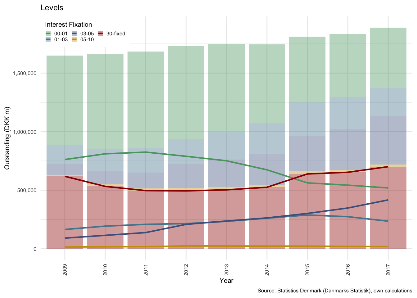
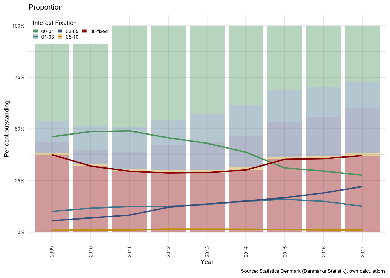
Figure 3.1: Mortgage debt in Denmark: All term lengths

This can also be considered in proportional terms, where the percentage of debt outstanding in each category is easier to read. As can be seen in Figure part (b) above, the 30-fixed category, which covers all fixed rate products¹⁹, was still in decline as a proportion of total outstanding mortgage debt from 2009 to 2012.

The most concerning factor, and one raised by Sheehy (2014), in an IMF stability report, was the growing proportion of debt that would reprice within relatively short intervals. At the start of 2011, debt with an interest fixation of less than and up to 1 year (the green line) was by far the largest contributor. This was recognised by both domestic and foreign prudential regulators as a risky development, and in collaboration with the banking sector and real estate finance companies a variety of measures were implemented to reverse this trajectory. (Sheehy 2014)

These patterns can further be decomposed into a variety of term structures. As can be seen from Figure , the proportional composition of debt is significantly different for each of the term groupings²⁰. We will not explore this too deeply, as the relative importance of each category varies dramatically.

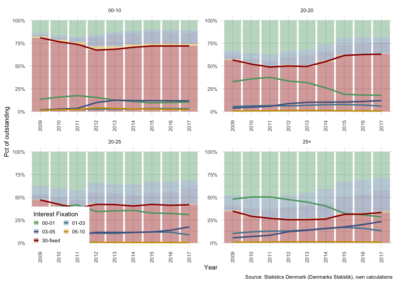
Figure 3.2: Composition of mortgage debt in Denmark: Split by term

Figure illustrates the total outstanding debt in each of the term categories, it can quite easily be seen that by far the largest portion of debt has a term to maturity of over 25 years. In Denmark, the maximum term for which mortgage debt can be acquired is 30 years, thus all debt in this category in each year was issued under five years prior to the year in question. Roughly only one sixth of all outstanding mortgage debt has a term to maturity of less than 25 years.

Of the debt with greater than 25 years to maturity, it can be seen from Figure , that only approximately 30% of this outstanding debt has an interest fixation period of longer than 5 years. This together with approximately half of the other 15% results in a total of just over 37% of all outstanding mortgage bond debt. This means that the remaining 63% of mortgage debt will adjust together with interest rates. The outstanding mortgage bonds will also adjust in price, which effectively means that in the event of an increase in interest rates, nominal debt outstanding will remain fairly constant for the 63% that has flexible interest products, and debt service costs will rise commensurate with the rise in rates. The aggregate opportunity cost related to capital adjustments for borrowers in this case is potentially very large.

By 2017, the proportion of debt with an interest fixation period of 1 year or less had fallen to approximately 25% of all outstanding debt. A significant improvement from just under 50% for 2010 and 2011.

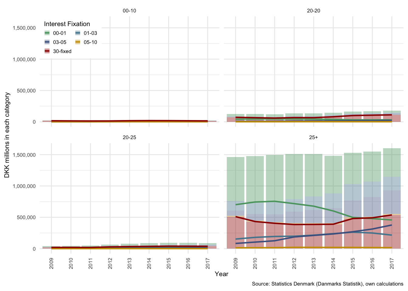
Figure 3.3: Levels of mortgage debt in Denmark: Split by term

Based on the distribution that can be seen in Figure above, the remainder of the paper uses a much simpler term and interest fixation categorisation. In order to capture all long term debt, all outstanding debt with a term longer than 10 years is included in long term debt, while all shorter terms maturity are included in the short term category. Similarly, interest fixation periods of less than 10 years are included in the short fixation period category, of which the overwhelming majority is fixed for less than five years. All interest fixation periods of longer than 10 years are included in the fixed-interest category. Because the level of mortgage debt with a shorter term is so low (largely irrelevant), this additional categorisation is dropped. Any shorter term mortgage debt is also likely to have similar characteristics of longer term debt that has short interest fixation periods. As such, it is assumed that the only fixed interest debt held by HH is held in the form of mortgage debt. It is therefore possible to categorise all debt in terms of the “interest fixation” dimension.

This is supported by Figure , where the proportion of debt in the shorter term category is essentially negligible in comparison with the longer term outstanding portion.

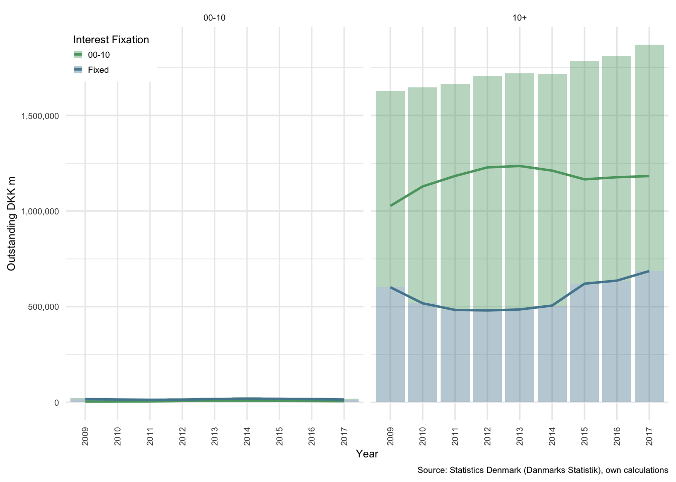
Figure 3.4: Composition of mortgage debt in Denmark: Simplified, panels by term

Figure shows the nominal outstanding amounts in the short and long term to maturity categories. As can noted above, the short-term-to-maturity debt to the left is of negligible interest for the analysis that follows, and so most of the figures below focus purely on the long term-to-maturity (10+ category) to the right.

Figure , part (a), reflects the relative proportions of fixed and flexible-interest fixation periods in each interest fixation category. The debt with interest-fixation periods of less than 10 years will be referred to as adjustable rate mortgages (ARMs) or flexible-rate mortgages below.

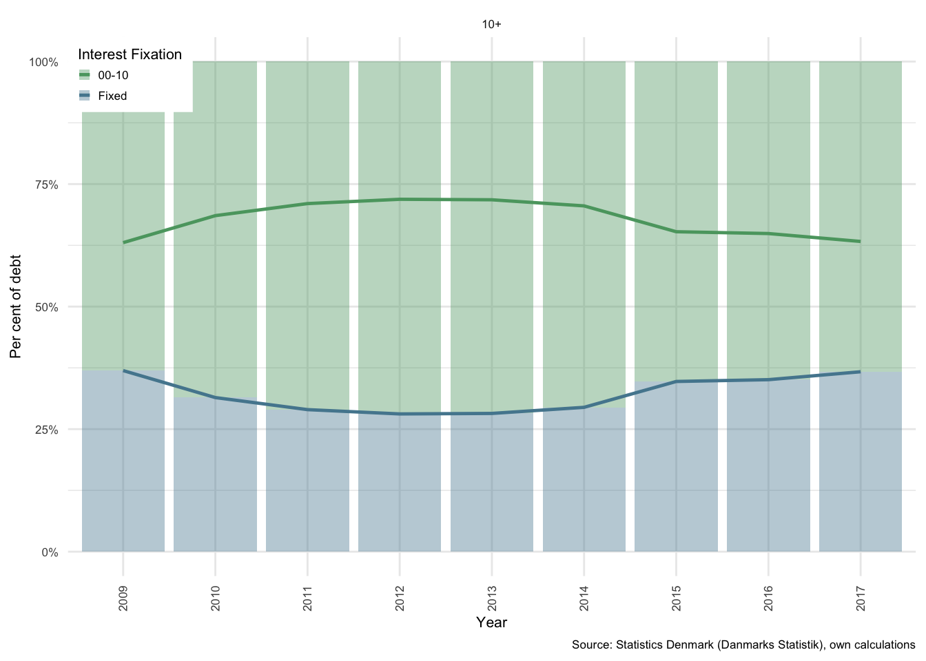
Figure 3.5: Outstanding mortgage debt and interest payments: Term of 10+ years

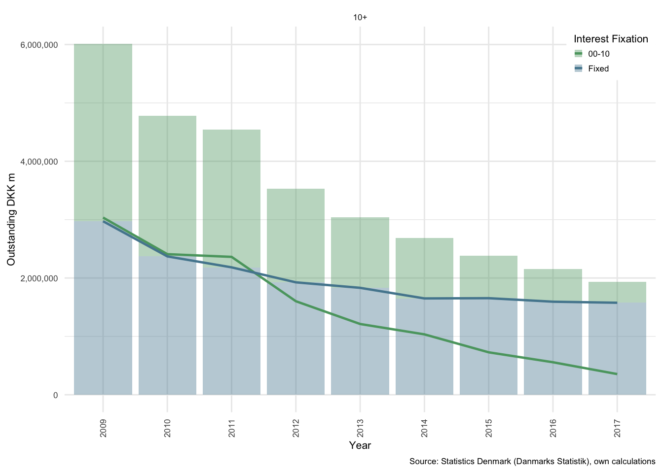
Figure 3.6: Interest payments

The cost of the outstanding debt has not followed the same pattern. Figure part (b) above, shows that the total interest expenses paid on shorter ARM debt has declined in nominal terms from roughly equivalent to the fixed-interest debt in 2011 to just a fraction of total interest paid on fixed-interest products by the end of 2017.

This can then be represented as an average rate of interest by calculating the amount paid divided by the total outstanding debt. In Figure , the short-term-to-maturity characteristics are shown on the left to illustrate the these products follow market rates more closely. Again, however, it is the panel to the right that we are most interested in, where it is possible to see that longer term ARM debt paid an average rate of just under 0.5%, while fixed rate longer term debt paid on average approximately 2.4% in 2017. The spread has interestingly remained relatively constant between the two average rates, but the proportional decline in the ARM average rate has been approximately -86%, while the same for fixed rate products has been approximately -50%. It appears, from this illustration, that a fall in official interest rates has passed through to mortgage markets at roughly the same speed in fixed and ARM products²¹.

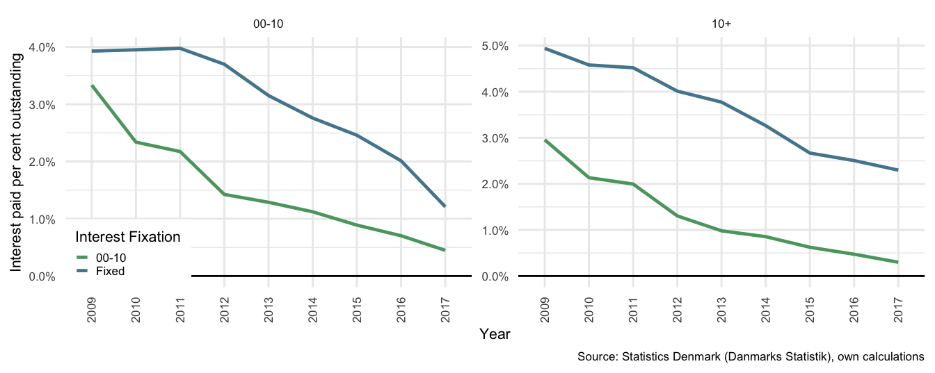
Figure 3.7: Interest paid per cent of mortgage debt outstanding: By term

As can be expected, in the Danish environment, as interest rates fall and the option to refinance remains available to households, the rate of interest on fixed-interest securities has followed the flexible rate of interest downwards - with a relatively constant spread of approximately 2% points. Unfortunately we do not have data on how this spread alters during a rising interest rate period. It can be seen that there was some delay in convergence in shorter terms to maturity. This is expected as the costs associated with refinancing existing contracts are likely to outweigh the benefits of a reduction in interest expense on smaller capital values, or on products with shorter terms to maturity (i.e. fewer interest payments remaining).

In a rising rate environment borrowers again have the incentive to refinance in order to take advantage of falling bond prices, since in Denmark the borrower has the option to either pay back the cash capital value or to repurchase an equivalent bond to the one issued on the date of borrowing (otherwise known as a prepayment or buy-back option). If interest rates rise sufficiently to make it profitable, and if they have accumulated sufficient equity, the borrower has the opportunity to make a substantial reduction in the outstanding capital amount. Thus, unless rates remain unchanged, or only vary marginally, for an extended period of time, the proportion of outstanding debt that has been recently refinanced will typically be quite high²².

3.3.0.2 Affordability of debt

The debt-service ratio (DSR) is shown in Figure , and calculated as the ratio between total outgoing property income payments to annual HH disposable income. In aggregate terms, it is unsurprising that the DSR has fallen continuously for the Danish household sector since the GFC. It is presently at the lowest level since 1995, and according to data collated by Abildgren (2017), the lowest level ever. Thus in relative terms, while debt may be at record high levels relative to income, the aggregate cost of servicing that debt is at an all time low.

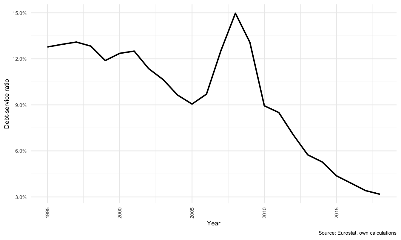
Figure 3.8: Debt-service ratio: Denmark

This paradox between the level of debt outstanding and the declining DSR is discussed in analysis in Section The implications for the economy as a whole and for the household sector depend on the macroeconomic linkages between the sectors and the drivers of agent decision-making in the model structure.

3.4 The model

The model implemented in this section is based on Byrialsen and Raza (2019), which is at the time of writing the most advanced empirical Stock-Flow-Consistent (SFC) macroeconomic model of Denmark. The full model together with an explanation for each equation and the logical connections between each of the sectors, flows and stocks is provided in Section , in the appendix.

Throughout this section some of the equations and explanations thereof are duplicated for explanatory purposes. It will provide only a brief summary of the core features of the model, and the highlight the main changes made for this analysis.

The model consists of the five main institutional sectors, namely the household sector (HH) non-financial corporate sector (NFC), the financial corporate sector (FC), the general government (G), and the rest of the world (ROW). It was developed between 2017 and 2019 with a focus on the Danish HH. As such, the behaviours of all sectors are significantly simplified, except in so far as they engage directly with HH. The model is fully empirical, in the sense that all variables included in the model are available as a dataset, against which the performance of the model can be tested.

One feature is worth noting up front. As mentioned in the introduction, the full model has 131 endogenous and 78 exogenous variables. Included in the exogenous variables are all rates of return and all financial asset prices. The most important implication is that correlated asset price and market movements are not endogenous in the model, and this limits the analysis to very short-term model responses.

3.4.1 Data

The data used for the model in this article is sourced from a combination of Eurostat data, OECD data, and AMECO data. The period for which annual data is available in sufficient detail is from 1995 to 2017. This data is then processed in a series of aggregations. The data and the model accounting structures follow the ESA 2010 (Statistical Office of the European Communities. 2013) accounting structure, and the contents of the financial balance sheet can be summarised as:

Monetary gold and special drawing rights (F1), Currency and deposits (F2), Debt securities (F3), Loans (F4), Equity and investment fund shares (F5), Insurance, pensions and standardized guarantee schemes (F6), Financial derivatives and employees stock options (F7) and Other accounts (F8). These data are aggregated according to Table .

Table 3.1: Aggregation of ESA balance sheet categories

Assets	Eurostat Code (ESA 2010)
Interest bearing (\(IB\))	\(F_1\), \(F_2\), \(F_3\), \(F_4\), \(F_7\) or \(F_8\)
Net interest bearing (\(NIB\))	\(F_1\), \(F_2\), \(F_3\), \(F_4\), \(F_7\) or \(F_8\)
Net equities (\(NEQ\))	\(F_5\)
Pension (\(PEN\))	\(F_6\)

The financial markets are thus highly aggregated in the model with effectively only three asset classes. \(IB\) covers all securities that provide a financial return that is analogous to interest, as does \(NIB\). The only difference is that for NFC, GOV and ROW, as part of the aggregation process, only the net position in these assets and liabilities are considered.

The other two major asset classes are equities and pension funds. All except HH equities are expressed as net equity assets and liabilities, \(NEQ\), and for HH they are expressed as equity assets, \(EQA\), as they cannot issue equity liabilities by definition. Pension assets are expressed as \(PEN\), and are recorded as net pension assets (\(NPEN\)) for ROW.

3.4.2 Major changes

The most significant change in this version of the model is the introduction of a split between fixed and flexible rate mortgage debt. This relatively simple alteration allows one to test the sensitivity of HH balance sheets to a change in debt composition. The drivers of debt remain the same, and the rates of return on all other assets have been left unchanged.

This is to isolate the channel through which the change in the cost of borrowing affects households in the short term. This makes it possible to identify the transmission channels and magnitude of each shock more clearly. It is one of the advantages of fully exogenous rates of return and asset prices, but comes at the cost of more realistic inter-market (“pass-through”) responses.

3.4.3 Balance sheet and transactions flow matrices

As with all SFC models, the balance sheet matrix represents the distribution of ownership of assets (\(+\)) and liabilities (\(-\)) in the modelled economy. As can be seen from Table , the sum of all rows, with the exception of fixed capital, are zero. This reflects that each asset (except fixed assets, \(K\)) is exactly offset by a liability held by another sector.

The financial asset classes mentioned above are assigned to each sector according to assumptions of which sector issues or holds each type of security. FC holds the majority of counterpart financial securities, and in all sectors except HH, financial assets and liabilities are recorded in net terms (assets minus liabilities).

The interest bearing liabilities of HH are, as noted in the previous section, by a vast majority, long term debt. This is separated into fixed-interest (\(IBL(FI)^F\)) and flexible-interest (\(IBL(FL)^F\)) (or, ARM) mortgage liabilities.

Horizontal consistency captures the idea that all accounts are recorded as dual entry accounting records, and the sum of all sector positions in any financial asset class should be zero. Vertical consistency represents the financial position of each sector, where financial net wealth (\(FNW\)) is the sum of all assets and liabilities and will either be a net positive or negative value. The sum across sectors of the \(FNW\) of all sectors is also zero.

Table 3.2: Balance sheet matrix: BSM

Stocks	NFC	FC		GOV	HH		ROW	\(\Sigma\)
		Assets	Liabilities		Assets	Liabilities
Financial Stocks
Interest bearing (IBA / IBL)			\(-IBL^{F}\)		\(+IBA^{H}\)			0
Interest bearing Fixed		\(+IBA(FI)^{F}\)				\(-IBL(FI)^{H}\)		0
Interest bearing Flexible		\(+IBA(FL)^{F}\)				\(-IBL(FL)^{H}\)		0
Net interest bearing (NIB)	\(NIB^{N}\)	\(NIB^{F}\)		\(NIB^{G}\)			\(NIB^{W}\)	0
Net equities (NEQ)	\(NEQ^{N}\)	\(NEQ^{F}\)			\(NEQ^{H}\)		\(NEQ^{W}\)	0
Pensions (PEN)			\(-PEN^{F}\)		\(+PEN^{H}\)		\(NPEN^{W}\)	0
Fixed Stocks
Financial net wealth (FNW)	\(FNW^{N}\)	\(FNW^{F}\)		\(FNW^{G}\)	\(FNW^{H}\)		\(FNW^{W}\)	0
Fixed assets (K)	\(K^{N}\)	\(K^{F}\)		\(K^{G}\)	\(K^{H}\)			\(K^{T}\)

The transactions flow matrix is presented below. This matrix, much like the balance sheet matrix presented above, observes the requirements of horizontal and vertical consistency. In this table, all items that result in a positive flow of funds for the sector in question are marked with a plus sign (\(+\)), and all those that result in a flow outwards of funds are marked with a minus sign (\(-\)).

The expenditure approach to GDP is captured in the first five lines of the table, and can be captured as,

\[\begin{equation} Y = C + I + G + (X - M) \label{eq:gdp_intext} \end{equation}\]

Where \(C\) is consumption, \(I\) is investment, \(G\) is government expenditure, \(X\) is exports and \(M\) is imports. All in nominal terms to reflect the actual flows of funds in each period. The income approach to national expenditure is captured in the following six lines in the table up until the row called Savings. Each row name reflects the flow that is applicable to each sector. The full detail of how these flows are defined can be found in the full model description in Section , in the appendix.

Capital income (\(rK\)), transfers (\(STR\)), capital transfers (\(KTR\)), acquisitions less disposal of fixed assets (\(NP\)) and net lending (\(NL\)) are presented without a particular sign attached to each sector. The reason for which is that each sector both receives and pays social transfers, and although GOV is the primary counterpart for all of these, the size and net sign of these transfers can change over time. The same is true for \(KTR\) and \(NP\). Net lending (\(NL\)) is a passive (residual) value and is determined by the balance of funding requirements between the sectors over time, and can therefore also swing between negative or positive as a flow.

Table 3.3: Transactions flow matrix: TFM

Flows	NFC		FC		GOV		HH		ROW		\(\Sigma\)
	Current	Capital	Current	Capital	Current	Capital	Current	Capital	Current	Capital
Private consumption	\(+C\)						\(-C\)				0
Government consumption	\(+G\)				\(-G\)						0
Investment	\(+I\)	\(-I^{N}\)		\(-I^{F}\)		\(-I^{G}\)		\(-I^{H}\)			0
Exports	\(+X\)								\(-X\)		0
Imports	\(-M\)								\(+M\)		0
GDP	Y										0
Taxes	\(-T^{N}\)		\(-T^{F}\)		\(+T^{G}\)		\(-T^{H}\)		\(-T^{W}\)		0
Gross operating surplus	\(-B2^{N}\)		\(+B2^{F}\)		\(+B2^{G}\)		\(+B2^{H}\)				0
Wages	\(-WB^{N}\)						\(+WB^{H}\)		\(WB^{W}\)		0
Capital income	\(rK^{N}\)		\(rK^{F}\)		\(rK^{G}\)		\(rK^{H}\)		\(rK^{W}\)		0
Transfers	\(STR^{N}\)		\(STR^{F}\)		\(STR^{G}\)		\(STR^{H}\)		\(STR^{W}\)		0
Pension adjustments			\(-CPEN^{F}\)				\(+CPEN^{F}\)				0
Savings (per sector)	\(-S{N}\)	\(+S{N}\)	\(-S{F}\)	\(+S{F}\)	\(-S{G}\)	\(+S{G}\)	\(-S{H}\)	\(+S{H}\)	\(-S{W}\)	\(+S{W}\)	0
Capital transfers		\(KTR^{N}\)		\(KTR^{F}\)		\(KTR^{G}\)		\(KTR^{H}\)		\(KTR^{W}\)	0
Acquisitions less disposal FA		\(NP^{N}\)		\(NP^{F}\)		\(NP^{G}\)		\(NP^{H}\)		\(NP^{W}\)	0
Net lending		\(NL^{N}\)		\(NL^{F}\)		\(NL^{G}\)		\(NL^{H}\)		\(NL^{W}\)	0
\(\Sigma\)	0	0	0	0	0	0	0	0	0	0	0

The three rows after the Savings row illustrate adjustments to the level of savings (\(S\)) as a result of capital transfers (\(KTR\)), purchase and sale of fixed assets (\(NP\)) and (from the third row of the table) the level of investment (\(I\)) of each sector - summed vertically in the capital accounts column for each sector. The sum of all of these items is reflected in a net financing requirement for each sector, in the table is called Net lending. The sum of all net lending positions in the economy is again necessarily equal to zero, as one sector’s surplus is at least one other sector’s deficit. The sum of all columns and all rows are thus all equal to zero, and this criterion is respected by the data collected from Eurostat on an annual basis.

Financial and fixed assets in the model are subject to both transactions and revaluations (or capital gains or losses). The accumulation of certain types of assets or liabilities depends in part on the action of the sector in question and in part on the effects of the other sectors. As can be read in the full model description in the appendix, the nominal values that are sourced from the Eurostat database and or AMECO can then be deflated using appropriate price indices. There are 19 different price indices used in the model, some of which are calculated, but the majority of which are sourced either from Statistics Denmark, AMECO or the OECD. The details of the model structure and the performance of the model relative to the data available can be found in Byrialsen and Raza (2019), and the details of the behavioural equations available in Section , in the appendix.

What we are most interested in here, however, is the specific channels through which the scenarios proposed below transmit. As mentioned above, the model contains active behaviours and passive behaviours. In each period, in order to ensure closure in the model, there is one variable in each sector that is passive to the budget constraints of each year.

The passive accumulator flows (or residual, buffer variables) for each sector are as follows: transactions in net interest bearing securities for NFC (\(NIBTR^N_t\)), GOV (\(NIBTR^G_t\)), and ROW (\(NIBTR^W_t\));and, transactions in interest bearing assets for HH (\(IBATR^H_t\)). While specific behavioural equations determine the holding of all other financial assets, \(NIB\) securities act as a catch all category for NFC, GOV and ROW. The sum of those positions is then absorbed by FC. As will be discussed below, the final closure of the model is provided through the indirect provision of equity assets to HH by FC on demand. This is fitting, since HH purchases of mutual funds or unit trusts are likely to be fulfilled by FC, rather than directly by NFC.

3.5 Scenarios

This section briefly explains the four scenarios investigated using the model. Apart from alterations to the structure of household mortgage liabilities, the model operates in the same manner as in Byrialsen and Raza (2019). The shocks presented below are measured as a percentage change from the baseline scenario. This allows for a simpler comparison between scenarios, and the aggregate nominal and real values of stocks and flows are illustrated where relevant.

The first shock (and Scenario 1) is an increase in interest rates in 2020, the second shock (and Scenario 2) is a decline in property prices in 2022. Scenario 3 compounds the first two, in that the first shock is kept in the model before the shock to property prices is imposed. The last scenario, Scenario 4, is a reduction in the level of ARMs in 2017. Effectively, the last scenario changes the pre-conditions for the first two shocks, but applies them in exactly the same manner. It is therefore possible to make a direct comparison between Scenario 3 and Scenario 4, given two different starting points.

This ordering allows the answer to a counter-factual question: What if HH had not taken on as much flexible rate mortgage debt? How would this shift in interest rate exposure affect outcomes, both for HH and the broader economy? In essence, what might have been the case if the innovations leading up to 2003 had not impacted borrowing decisions to the same degree? There are however, some limitations to the current model that are relevant for this exercise.

3.5.1 Limitations for interpretation of results

Adjustable Rate Mortgages (ARMs) typically do not adjust immediately

As noted above, the bulk of ARMs in Denmark adjust fewer than 5 years into the future. This allows households an extended period of time to observe interest rate fluctuations and make a decision regarding refinancing or property sale. It also means that the effects of an interest rate change will only impact HH cash flows after between one and five years.

A decline in house prices is unlikely to happen in isolation

A fall in house prices is not expected to occur in isolation. Unlike in the model below, a collapse in property prices is unlikely to be an isolated event. It would more likely accompany broader systemic problems or be triggered by some form of financial or economic crisis.

The structure of the economy at end 2017 is integrated with the volume and structure of household debt

For the fourth scenario, it is assumed that we can simply shift the structure of debt and leave the remainder of the economy unchanged. In reality, the total level of debt outstanding would probably be significantly lower if ARM and interest-only products had not been made available. This would have affected a significant array of economic variables, not least of all, domestic demand and house prices. Although this is true, HH have already accumulated significant levels of debt. As such, Scenario 4 is less a question of, what if things had been different, and more a question of how to structure policy in order to best influence future refinancing decisions of HH.

Interest rate changes would change the composition of debt

Refinancing in response to interest rate changes in Denmark is extensive. In a rising interest rate environment, the incentive is to repurchase the previously issued bond at a reduced price, settle the older debt, and then refinance at similar monthly instalments, but with a lower capital value outstanding.

With falling interest rates, the incentive is to refinance at lower monthly instalments, and if possible using a bond with fixed-interest, thus creating the opportunity to refinance if rates rise significantly in the future, and thus reduce the level of debt outstanding. It is therefore unlikely that the structure of debt would remain constant after a shift in rates²³. Due to the costs involved in refinancing, a change in interest rates is expected impact debt structures gradually, remaining fairly stable for the first year or two, and adjusting to a greater degree in the medium term (approximately up to 5 years).

3.5.2 Scenario 1 - An increase in interest rates

The first shock is a simple interest rate change. The point is to illustrate the expected impact on the level of household disposable income and the household balance sheet.

In this shock we consider a 2 percentage point (\(2\%\) points) rise in official rates. This is assumed to be passed through perfectly to ARM mortgages (interest rate on flexible-interest-rate mortgage debt, i.e. flexible rate products, with subscript (FL), (\(r^H_{L(FL)_{t}}\)). The cost of fixed-interest mortgage debt (\(r^H_{L(FI)_{t}}\)) is increased by a proportionally lower adjustment of point five percentage points (\(0.5\%\) points) to reflect lower sensitivity of adjustments of the overall stock of fixedinterest rate products. This is a strong assumption, and is not likely to hold over longer periods of time, fixed-interest rate debt holders are expected to retain their debt at lower interest rates, while the majority of flexible-interest rate holders are expected to participate fully in the rise in interest rates after a period of three years²⁴.

In the model baseline, the current rate is calculated as interest payments relative to outstanding debts. This gives a weighted average at the end of 2017 of 1.41% for all debts²⁵. After the shock, the adjustment is from this average rate upwards - thus flexible-interest rates are adjusted up to 2.41% and fixed-interest rates up to 1.91%. This constitutes a 141.75 per cent increase in flexible rates, and taking into account changes in the level of outstanding debt in 2021, a 136.29% increase in interest payments. For fixed-interest debt, it constitutes a 35.44 per cent increase in fixed rates, and a 32.38% increase in interest payments.

The interest rates in the model include, interest on fixed (\(r^H_{L(FI)}\)) and flexible rate (\(r^H_{L(FL)}\)) mortgages, and the counterpart assets (\(r^F_{A(FI)}\), \(r^F_{A(FL)}\)), the general rate of return on net interest bearing assets (\(r_{N}\)), and the return on interest bearing assets for households (\(r^H_{A}\)). The other rates of return are the domestic and foreign rate of return on equities (\(\chi _t\)), and pension assets (\(\psi _t\)). All rates of return in the model are determined exogenously, which means that any adjustment must be applied manually. As noted above, the change is limited to the cost of borrowing for HH only.

In the case of household debt, it is FC that holds the counter-balance assets. Thus,

\[r^F_{A(FI)_{t}} = r^H_{L(FI)_{t}}\] and, \[r^F_{A(FL)_{t}} = r^H_{L(FL)_{t}}\]

FC receives \(r^F_{A(FI)_{t-1}}(IBA^{F\sim H}_{A(FI)_{t-1}})\), and the two interest rates are simply made equivalent. An increase in rates results in an increase in costs for HH and an increase in revenues for FC.

Figure illustrates, in part (a) the actual monthly interest rates available for new debt on Danish mortgage markets since 2013 (separated by term of interest fixation). Part (b) shows the progression of official interest rates in Denmark since 2000, where the “Mortgage bond” rate is the dark-red line, and is comparable with Fixed mortgage bonds in panel (a), the purple line, from 2013 onwards. Part (c) illustrates the impact of the shock to interest rates in the model in 2020.

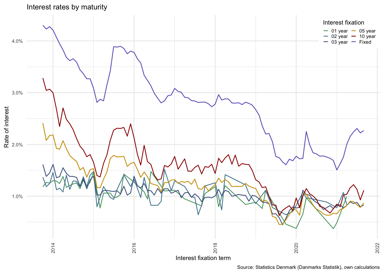
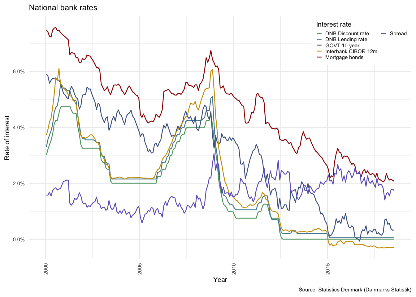
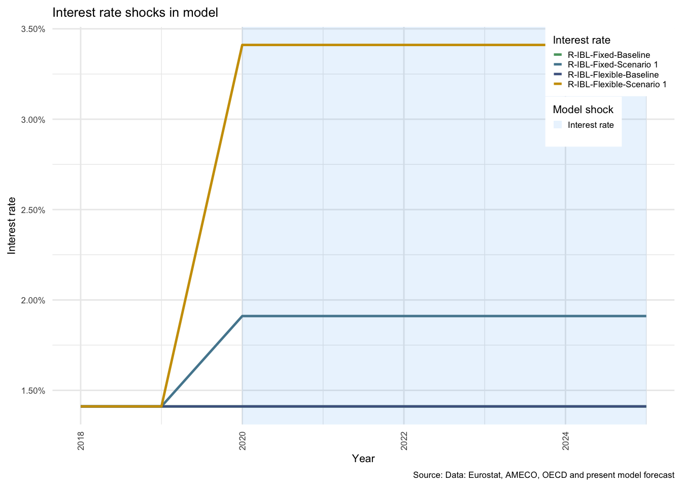
Figure 3.9: Interest rates in Denmark

As can be seen from part (a), the rates available to fixed rate borrowers have followed market rates downwards throughout the period, although this illustrates only those rates available, rather than those paid. Figure showing the amounts actually paid in the section above, however, illustrates that the amount paid has also declined at a similar pace, although with a marginal delay.

The interest rates in the model are split into fixed and flexible rates for the purpose of testing the effects of a shock to interest rate on alternative compositions of mortgage debt. The baseline value of interest rates remains just below 1.5% on average for all debt.

The expected outcome is that where the proportion of fixed-interest outstanding debt is higher, the effects of a shock will be weaker, and vice versa. This of course can only have an impact in the case where mortgage debt is itself split into fixed- and flexible-rate debt.

The total level of outstanding \(IBL\) for HH is split into fixed-interest (\(IBL_{FI}\)) and flexible-interest bearing liabilities (\(IBL_{FL}\)). The proportion of interest bearing assets held as \(IBL_{FI}\) is \(\alpha\).

\[\begin{equation} IBL^H_{{FI}_t} = \alpha(IBL^H_t) \end{equation}\]

and thus,

\[\begin{equation} IBL^H_{{FL}_t} = (1-\alpha)(IBL^H_t) \end{equation}\]

The level of \(\alpha\) is calculated from data acquired from multiple data sources at Statistics Denmark, and varies over time. The split was first introduced in 1996, but initial volumes were low. As discussed in Section , while the composition of this debt is significantly more complex than this, a strong argument can be made for an aggregation up to just these two categories. This split has no effect on the model prior to the shock in 2020, as the rate of interest on each is considered to be equal to the average rate used in the baseline scenario up to that point.

It is also possible to shock all other rates of return to a similar degree. Given the integration of financial markets, this would produce results in the model that are more realistic. Unfortunately, it would also conceal the effects that are purely due to dynamics linked to the interest cost of borrowing for households²⁶.

3.5.3 Scenario 2 - A fall in house prices

The second scenario is a fall in house prices. This is effected through a negative twenty per cent adjustment to the house price index (\(-20\%\)). This is a large change to house prices, but is equivalent to the stress test applied by the IMF (Sheehy 2014). At a national level, Figure illustrates that the average nominal house price index (HPI) for dwellings in Denmark has risen at a relatively steady pace since the GFC.

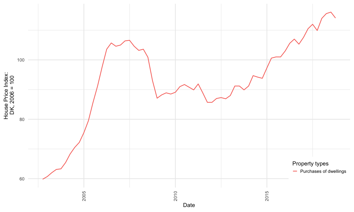
Figure 3.10: National House price index (HPI), 2006 = 100

This follows a collapse of house prices during the GFC, where prices of Danish dwellings fell approximately 20% from the peak in 2006 to the trough in 2011. This average was not uniform across property types or regions. As shown in Figure , the prices of owner occupied flats in the Capital and North Denmark Regions have risen at roughly the same pace as prior to the GFC. This is not predictive of a correction or price collapse, but does suggest a possible housing price bubble in those markets. All other regions, appear to have only just recovered to pre-crisis prices²⁷.

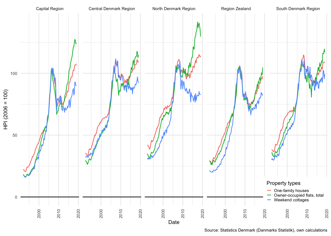
Figure 3.11: House price index (HPI), 2006 = 100

A more serious concern for potential borrowers is that several markets, particularly those for weekend cottages (otherwise known as summer houses) have not recovered in the period following the GFC. Thus, any property purchased between 2005 and the collapse in 2007 would have a high probability of falling into negative equity²⁸.

In this model, households are only permitted to make productive investment in housing, which, as in G. Zezza (2008), Fontana and Godin (2013) and Beckta (2015), is considered only as a primary market. The major difference here is that households are assumed to produce the houses, whereas firms are housing producers for all three of the above-mentioned studies. The secondary market for houses is assumed to affect prices, but not the demand for additional housing investment. Demand for housing investment is determined by by a Tobin’s-Q-like function, partially driven by changes in disposable income and previous period housing investment, and partially driven by a relative shift in sales price (\({P^H_{t-i}}\)) and construction cost (\({P^i_{t-i}}\)) indices.

Real investment in fixed assets (dwellings), in Equation , is estimated as a log-linear function that depends on conditions in previous periods. This assumes that the decision to invest in houses occurs based on recent developments, but that actual changes in investment in fixed assets takes some time to materialise. It thus takes one period before the effects of the house price shock can be observed.

\[\begin{equation} ln(i^H_t) = \beta _i + \beta _i ln(i^H_{t-i}) + \beta _i ln \Bigg( \frac{P^H_{t-i}}{P^i_{t-i}}\Bigg) + \beta _iln(yd^H_{t-i}) \label{eq:realhousinginvestment_intext} \end{equation}\]

The shock imposed on the model is to the numerator of the Tobin’s Q ratio²⁹. The imposed decline in house prices affects sales prices negatively, relative to the cost of production, and thus has a contractionary effect on the Tobin’s q ratio, \(\Bigg(\frac{P^H_{t-i}}{P^i_{t-i}}\Bigg)\), and thus on HH real investment (\(i^H_t\)). The shock is implemented as a permanent decline in prices, and thus changes the value of the ratio for all periods following the shock. Growth in house prices continues according to the same trajectory as in the baseline in order to make for a more effective comparison.

The nominal level of investment in housing can be calculated by inflating the real investment in housing series (\(i^H_t\)) by the investment price index (\(P^i_t\), which is sourced from Statistics Denmark):

\[\begin{equation} I^H_t = i^H_t(P^i_t) \end{equation}\]

The nominal stock of housing (\(K^H\)), as with other assets to come, follows the simple process of previous stock (\(K^H_{t-1}\)), plus acquisition (in this case investment in new houses), less depreciation (\(D^H_t\)) plus capital gains (\(K^H_{CG_t}\)).

\[\begin{equation} K^H_t = K^H_{t-1} + I^H_t - D^H_t + K^H_{CG_t} \label{eq:nominalhoushingcapital1} \end{equation}\]

Capital gains on houses, in turn, can be calculated in an ex post manner as: \[\begin{equation} K^H_{CG} = \Delta P^H_t (K^H_{t-1}) \end{equation}\]

Which is simply the change in the price of houses applied to the level of stock at the end of the preceding period.

The change in house prices (\(\Delta P^H_t\)) leading into the current period is then by definition the same ratio proportion of capital gains to previous housing capital.

\[\begin{equation} \Delta P^H_t = \frac{KH_{CG}}{K^H_{t-1}} \label{eq:changehouseprice_intext} \end{equation}\]

Nominal housing capital held by HH at the end of the current period can be expressed as the price adjusted stock at the end of the previous period, plus net investment and depreciation. Equation is effectively a restatement of Equation , but with greater emphasis on the variable shocked in the analysis.

\[\begin{equation} K^H_t = K^H_{t-1}(1 + \Delta P^H_t) + I^H_t- D^H_t \label{eq:nominalhoushingcapital2} \end{equation}\]

The deflated real capital index can then be found, as in Equation () by dividing the series by the investment (housing) price index, from Equation ().

\[\begin{equation} k^H_t = \frac{K^H_t}{P^i_t} \label{eq:realhoushingcapital_intext} \end{equation}\]

Housing capital then forms part of HH net wealth, which feeds back into consumption decisions in subsequent periods. A decline in net wealth in period \(t\) leads to a decline in consumption in period \(t+1\).

The effects of changes in net wealth (\(NW\)), are then felt directly in the level of HH consumption, but with a lag on one period (as can be seen in Equation () in the appendix). Although a fall in house prices does not affect household disposable income to a substantial degree is contributes to a decline in overall economic activity, and therefore reduces the demand for labour in subsequent periods. This ultimately does affect household income but the effect is not as immediate as was the case for the interest-rate shock.

3.5.4 Scenario 3 - Combination of Scenarios 1 and 2

The third scenario consecutively applies the shocks from Scenarios 1 and 2. First the interest rate increase in 2020, and then the decline in property prices in 2022. This combination sets up the comparison to be introduced in Scenario 4 below.

3.5.5 Scenario 4 - Comparison for Scenario 3, proportion of fixed-interest debt 80%

The final alteration to the model is an increase in the proportion of mortgage debt held as fixed debt (\(\alpha\)) from the 2016 level of 33.42% up to 80% in 2017. This shift allows us to test the hypothetical difference of the impact of a shock to interest rates in an artificial scenario, where the proportion of flexible debt amounts to only 20% of outstanding household mortgage liabilities.

3.6 Simulations

This section explains the transmission of the two shocks in the scenarios described above. First, the components of the economy that are most dramatically affected are identified, and thereafter the key transmission channels that cause these effects are briefly discussed.

The key take-aways from this section are that shock 1 and 2 both propagate through the economy as described above, and that Scenario 3 results in greater volatility in the responses of the economy than Scenario 4. This has implications for the stability of the balance sheets of each sector and for the economy as a whole.

The effects of each shock are summarised in tables in Section for each of the above-mentioned scenarios³⁰. This approach allows a quick summary of the impacts of a shock. It shows all affected variables, and thus provides a snapshot of how broadly the shock propagates. One drawback is that it is a cross section in time, and thus is not able to show the progression of feedback effects over time. These tables are both used as a guide to the most important transmissions, and as a consistency check, to ensure that the model behaves within reason.

The model responds largely as expected to the first shock, with the exception of the rather extreme response of the financial sector. This is because FC transactions in net interest bearing assets (\(NIBTR^F\)) absorbs all financial transactions of the other sectors - or, stated differently, accumulates all financial imbalances. The second shock, to property prices, has a more interesting result with regard HH savings and will be discussed in more detail in the HH section below.

As noted above, each of the sectors has a buffer flow that summarises the collective effect of each shock, and each of the shocks are quite extreme in nature. It is therefore unsurprising that the effect on the passive elements is somewhat exaggerated. Even though shocks of the same magnitude have occurred in the past, they are not common events and have only been used here to enhance the potential risks associated with the different debt structures.

3.6.1 General economy

The first shock (to interest rates) has a delayed effect that is first visible in the shift from period 2020 to period 2021; as can be seen for Scenarios 1, 3 and 4. The second shock (to property prices) takes effect immediately in 2022, and can therefore be seen to take effect from period 2021 to period 2022 for Scenarios 2, 3 and 4. At a broader economic level, the strongest impact on the major components of GDP from the first shock are a decline in gross fixed capital formation (\(I\)) of -1.25% and in imports (\(M\)) of -1.22% (and as a result, net exports rise by just over 10.52%). Figure shows how \(C\), \(I\), \(G\), \(X\) and \(M\) would evolve relative to the baseline, for scenarios 1 and 2, and Figure that shows the same for Scenarios 3 and 4.

The shock to interest rates only impacts the model at \(t+1\) and so there is no change from the baseline in year 2020, whereas the impact of a property price shock takes immediate effect in 2022. Exports remain relatively unchanged under both shocks, only marginally affected due to a shift in domestic prices. \(Y\), or GDP, is more affected by the shock to interest rates in Scenario 1 than by property prices in Scenario 2, largely as a result of the limited impact of the property price shock on \(C\) and \(M\). The rapid rise in interest costs clearly result in a decline in all demand components except for \(G\), which is exogenous and therefore remains completely unchanged in all scenarios.

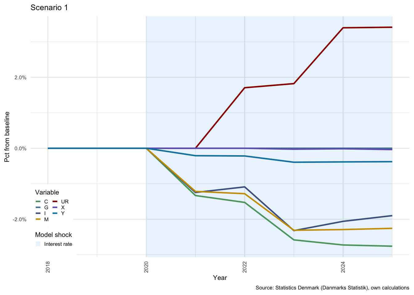
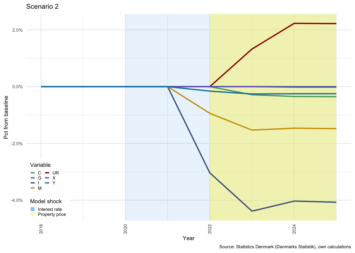
Figure 3.12: National income indicators - Scenarios 1 and 2

As described above, Scenarios 3 and 4 illustrate the compound effect of the two shocks under two different household debt positions. In Scenarios 1 to 3, proportion of fixed-interest debt (\(\alpha\)) is 38.91%, in Scenario 4, \(\alpha\) is set to 80%. The primary impact of this shift is a reduction in the sensitivity of household disposable income to a dramatic rise in interest rates.

As expected, the effects of the combination of the two shocks are significantly dampened when \(\alpha\) is higher. This is clear from the scales in Figure , where on the left for Scenario 3, investment drops just below -6% compared with -5.5% on the right for Scenario 4. This pattern repeats itself throughout this results section.

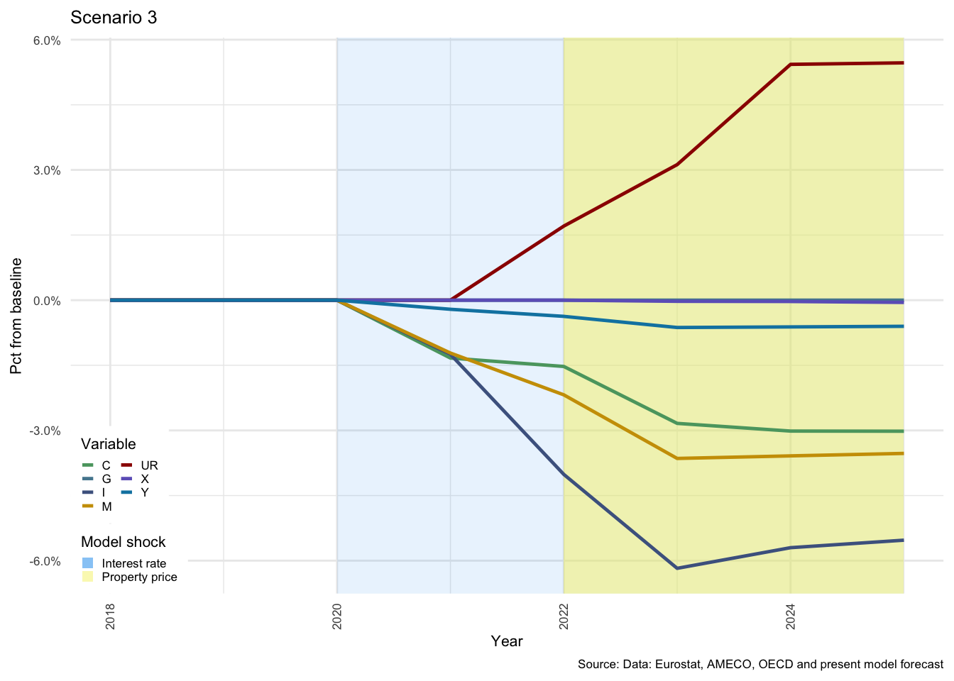
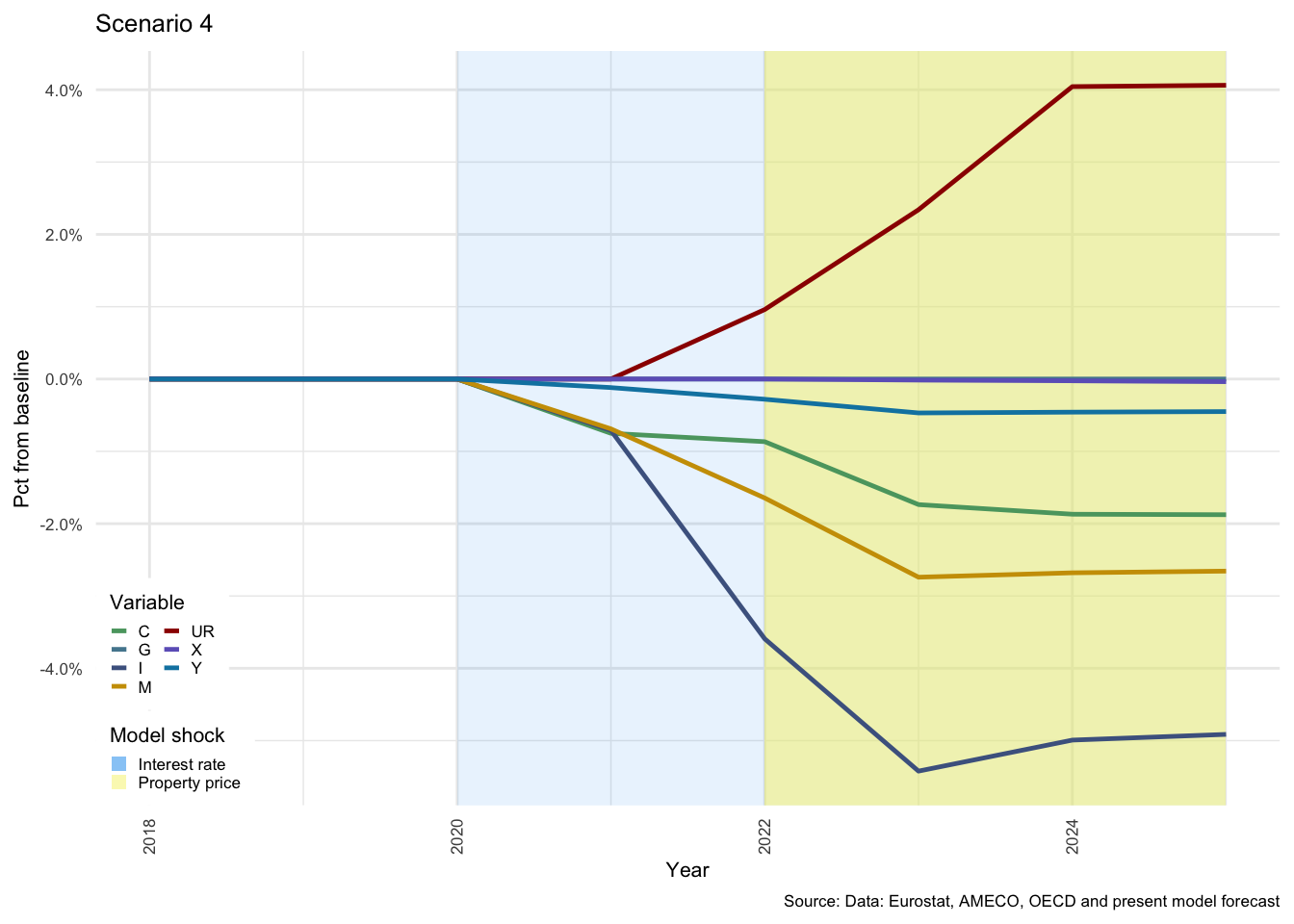
Figure 3.13: National income indicators - Scenarios 3 and 4

GDP is also somewhat better protected from the shock in the latter case. The unemployment rate (\(UR\)) increase is a compound effect of the two shocks, and is also significantly higher in Scenario 3 than in Scenario 4. The number of persons employed are determined by the NFC, and is a function of the level of \(Y\) in the previous period and changes in the size of the labour force. Exogenous growth in the size of the labour force combined with a decline in economic activity, drive the proportion of unemployed persons upwards. This also results in a rise in the level of social benefits drawn by HH from GOV, but this will be discussed in the sections for each sector below.

In many of the charts that follow, all scenarios are displayed for each of the variables. This allows for a comparison of the impact of the shocks. The baseline scenario is illustrated by a solid black line, Scenario 1 by a light-grey, dashed line. Scenario 2 by a medium-dark-grey, dashed line. Scenario 3 by the dark-grey short-dashed line and Scenario 4 by the red short-dashed line.

For each sector we will highlight the components that move most dramatically for shocks 1 and 2, and thereafter will focus on the comparative difference of these effects in Scenarios 3 and 4. This highlights the major transmissions for each shock in each sector. It also allows us to compare the impact of a hypothetical change in the allocation of debt between fixed- and flexible-interest rate products. Essentially we are able to show the impact of financial innovations, within the bounds of the assumptions discussed above.

A summary of the impact of the shocks, as captured by the net financing requirements (Net lending, \(NL\)) of each sector for each year following the shocks, can be seen in Figure .

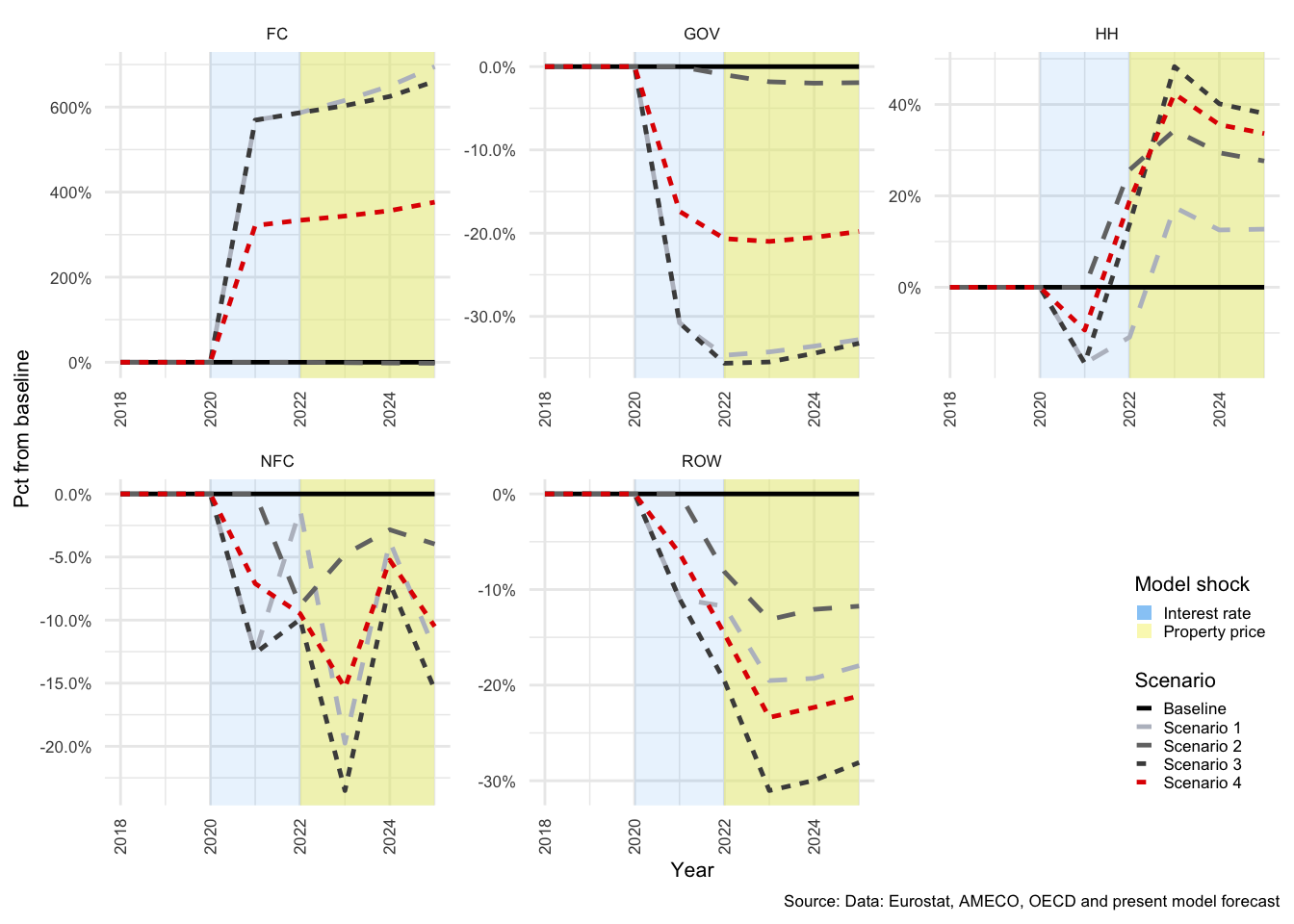
Figure 3.14: Net lending

Base purely on \(NL\), as shown in Figure , it would appear that HH are net borrowers (have negative \(NL\)) as a result of the interest rate rise, as might be expected, but rather counter-intuitively³¹ move into a strong net lending position following the property price collapse in 2022. ROW moves into positive \(NL\) in all scenarios, as does FC, with the exception of Scenario 2, which leaves FC \(NL\) unchanged. The scale of the changes in FC’s \(NL\) are a cause for concern, and will be addressed in the FC section below. NFC and GOV move into negative \(NL\) in all circumstances, but NFC has much more erratic movements.

For all sectors, Scenario 4 is again similar to Scenario 3, but with significantly less dramatic effects. The next section will help to highlight a problem with a focus purely on \(NL\). In summary, such a focus may not be indicative of the actual economic consequences of these shocks for each sector.

For each sector the analysis includes a brief summary the most affected components from each shock, plus a graphical analysis of the most important transmission channels. For Scenario 1, these can be seen in Tables to for (\(t + 1\)) 2021, and Tables to for (\(t+3\)), which is 2023.

For Scenario 2, they can be seen in Tables to for 2022, and Tables to for (\(t+3\)), which is 2025. Similar tables can be seen for Scenarios 3 and 4 from Table to Table , where the effects are summarised for the years 2021, which allows for a comparison of the first shock, and 2025, which captures the difference in the compound effect of both shocks.

3.6.2 Effects for the HH sector

For HH, in 2021, the most obvious effect of the first shock is the increase in interest paid on mortgage debt (or property income paid) of 95.85%. The immediate reduction in transactions for new interest-bearing assets (\(\downarrow IBATR^H\)) and liabilities (\(\downarrow IBLTR^H\)) by -78.28% and -73.94% respectively, and transactions in equity assets (\(\downarrow EQATR^H\)) fall by -68.34%. These are dramatic proportional shifts, largely due to the very low base of the baseline figures. These changes are not only driven by portfolio allocation decisions but also by changes in the real economy, as aggregate demand is reduced due tot he change in interest rates.

HH investment (gross fixed capital formation, \(\downarrow I^H\), which is only houses in this model) falls by -6.81% and savings by -10.3% (thus the decline in \(\downarrow NL\) of around -16.64%). This follows a decline in disposable income of -2.58% and consequently in consumption of about -1.33%. In terms of stocks, households immediately reduce holdings of IBL by -2.26% and IBA by -3.23%.

The residual financial flow for HH is transactions in interest bearing assets, \(IBATR^H_t\), which are assumed to be deposits. It is directly affected by changes in the level of net lending (\(NL^H\)), changes in transactions in IBL (\(IBLTR^H_t\)), transactions in equities (\(EQATR^H_t\)) and net transactions in pension assets (\(PENATR^H_t\)). The link between new debt \(IBL^H\) and new deposits \(IBA^H\) is analogous to the PK theory of endogenous money supply since an increase in debt is associated with an increase in deposits. This is represented in Equation .

\[\begin{equation} IBATR^H_t = NL^H + IBLTR^H_t - EQATR^H_t - PENATR^H_t \label{eq:ibatr_hh_intext} \end{equation}\]

The progression of each of these transaction flows is presented in Figure below. The decline in \(\downarrow IBATR^H\) of -78.28% is easily discernible. The reader should note that the scale on each plot differs, and the change to \(PENATR^H\) is largely irrelevant at less than 1%, and the declines in \(IBLTR^H\), \(EQATR^H\) and \(IBATR^H\) are of far greater interest. This is appropriate, as each item should be read independently.

Following the dark-grey dotted line describes Scenario 1, where, in all but pension asset transactions, the initial decline is dramatic, but in subsequent years there is a fairly rapid recovery. \(IBATR^H\) is represented in the top centre panel, and is the sum of the remaining four items. In Scenarios 1,3 and 4, the interest rate shock results in significant negative savings, but with the introduction of the property price collapse in 2022, for Scenarios 2 to 4, NL swings positive. This is explored further below.

Comparing Scenarios 3 (dark-grey short-dashed line) and 4 (red short-dashed line) reveals that the effect of the combination of the two shocks is 50% smaller for Scenario 4 after the interest rate shock (shock 1), and roughly 10% to 20% smaller for the property shock (shock 2).

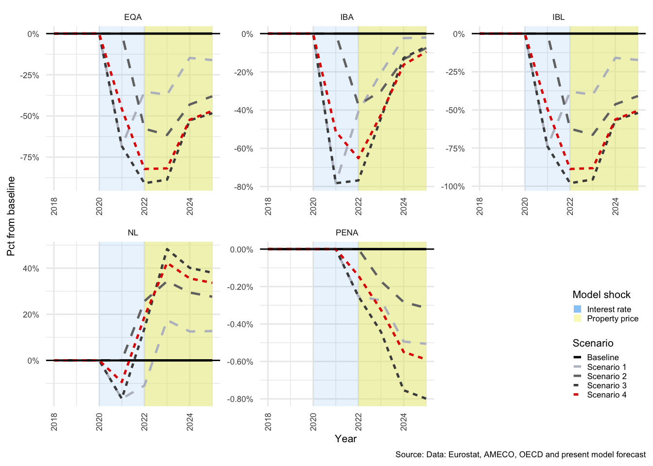
Figure 3.15: Households: Transactions in assets

The level of net lending \(NL^H_t\) is essentially driven by changes in savings (\(S^H_t\)) and investment levels (\(I^H_t\)). The changes in net purchases and sales of fixed assets (\(NP^H\)) and net capital transfers (\(KTR^H\)) are exogenous, and so do not differ from the baseline (this is repeated for all sectors). The level of net lending for HH is calculated as follows.

\[\begin{equation} NL^H_t = S^H_t - I^H_t - NP^H_t + KTR^H_t \end{equation}\]

The \(I^H\) and \(S^H\) components of \(NL\) can be seen in Figure . \(I^H\) (INV in the plot) recovers in the second period after the shock but then declines again in the fourth. \(S^H\) and \(NL\) fall by about around 10% in Scenarios 1 and 3, but only by about half of that for Scenario 4. \(I^H\) (which is entirely in houses) declines even more dramatically in Scenarios 2 with the collapse in house prices, and this is compounded with the fall of shock 1 in Scenarios 3 and 4. There is a decline of over 30% from baseline investment by 2023 when the level of ARM (flexible-rate mortgages) is allowed to remain high in Scenario 3.

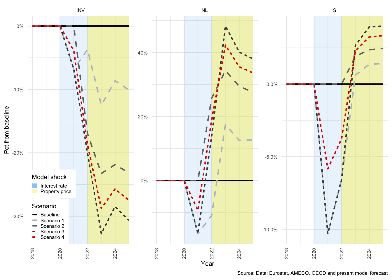
Figure 3.16: Household Net Lending components

Savings (\(S^H\)) are almost entirely determined by the level of disposable income of HH, and since the tax proportion is held constant, it is the income portion that drives most of the changes. While savings recover in the periods after the shock, investment activity declines further, which is the main driver behind the correction of \(NL\). Thus, it is unfortunately a decline in economic activity that allows for the financial recovery. The decline in \(I^H\) also means that capital formation fails to offset depreciation, and thus, HH capital levels decline.

Equation () describes the incomes and expenditures of HH that ultimately determine the gross income for the sector (\(Y^H_t\)). The primary sources of which are wages (\(WB^H\), W in the plot below), profits (\(B2\), which is exogenous), property income (or returns on financial capital, which stems from interest bearing assets, \(IBA^H\), pensions, \(PENA^H\), and equities, \(EQA^H\)), and social transfers (\(STR^H\), STRA in the plot below).

\[\begin{equation} \begin{split} Y^H_t = & WB^H_t + B2^H_{t} + r^H_{A_{t-1}}(IBA^H_{t-1})\\ & - r^H_{L(FI)_{t-1}}(IBL(FI)^H_{t-1})\\ & - r^H_{L(FL)_{t-1}}(IBL(FL)^H_{t-1})\\ & + \chi _t(EQA^H_{t-1}) + \psi _t(PENA^H_{t-1}) + STR^H_t + \epsilon ^H \label{eq:Yht-text} \end{split} \end{equation}\]

Interest rates are represented by \(r^H\), and the “A” (“L”) subscript referring to the assets (liabilities), and (\(\chi _t\)) and (\(\psi _t\)) are the rates of return on equities and pensions. As part of the key change in this model, the level of interest paid on \(IBL\) in this model is split between fixed and flexible rate mortgages into \(r^H_{L(FI)_{t-1}}(IBL(FI)^H_{t-1})\) (PIP-IBL-Fixed, in the plot below) and \(r^H_{L(FL)_{t-1}}(IBL(FL)^H_{t-1})\) (PIP-IBL-Flexible, in the plot below). A similar split is present in the financial corporate sector (FC) below.

The \(\epsilon ^H\) refers to adjustments made to ensure stock and flow consistency in the level of property income received or paid during the periods where data was available³².

Figure displays the endogenous components of HH income. Property income received on financial assets, are labelled PIR-EQA for \(EQA^H\), PIR-IBA for \(IBA^H\), PIR-PENA for \(PENA^H\). PIP-IBL is the sum of interest paid on \(IBL(FI)^H\) and \(IBL(FL)^H\), which is all interest paid on mortgage debt. Also included in the figure are consumption (\(C^H\)) and income tax (\(T^H\), TAX in the plot below).

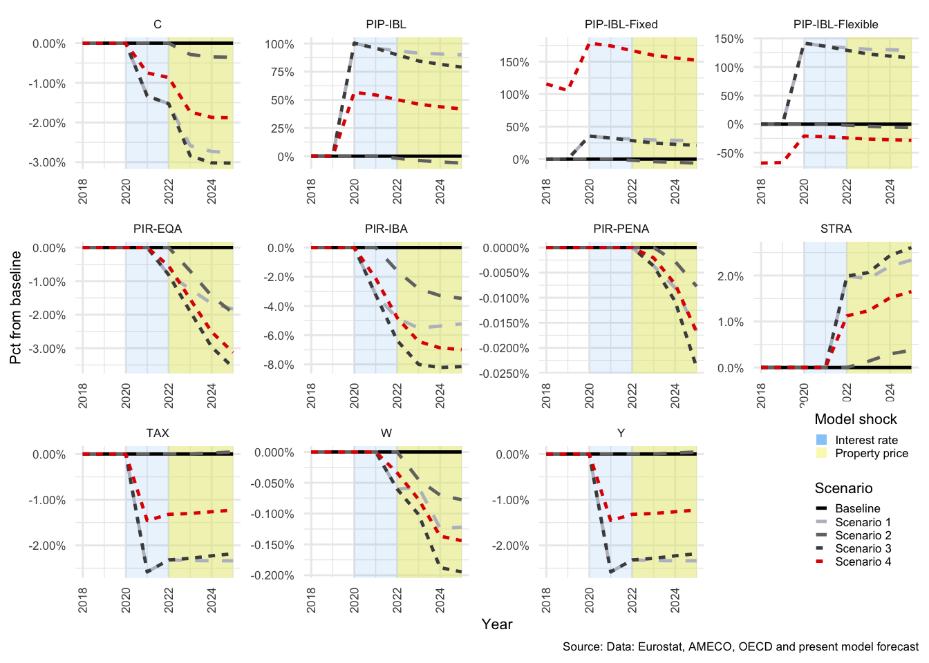
Figure 3.17: Household income components

The sum of all changes in the model accumulate in the level of \(Y^H\) in the bottom right hand panel of Figure , Scenario 2 has almost zero impact on \(Y^H\), while Scenarios 1, 3 and 4, which include the interest rate change, all result in a significant net decline. PIP-IBL, in the panel to the right of consumption (\(C\)) in the top left corner, is the total interest paid on debt by HH, and highlights the most dramatic change. It also illustrates the key difference introduced in Scenario 4, which is a reduction in the sensitivity of HH income to changes in interest rates relative to Scenario 3.

The largest contributors to HH income are wages (\(W^H\)) and social transfers (\(STR^H\), STRA in the plot above). Since 2007, approximately 35% to 37% of social transfers represent a tax funded pension income, and most of the remainder covers medical and disability support³³. To give a sense of scale, Figure shows the actual values of the major contributors, where NPIR is a net sum of all property income received and paid, and remains positive, but falls by roughly 50% due to the rise in interest costs on mortgages³⁴.

Wages (\(W\)), taxes (\(T^H\), TAX) and consumption (\(C\)) all decline with \(Y^H\).

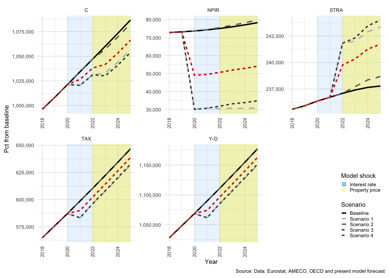
Figure 3.18: Household savings components

From this it is possible to see that the rise in \(STR^H\) is not sufficient to offset the fall in property income. Scenario 2 is the obvious exception, where income rises marginally. Disposable income (\(Y_d\), shown as Y-D above) declines in Scenarios 1 and 3, but in Scenario 4 only stagnates before trending upwards again. The trend in consumption follows the shift in \(Y_d\). The effects of the shocks on the HH financial balance sheet can be seen in Figure .

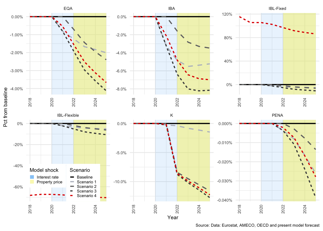
Figure 3.19: Household balance sheet

The decline in \(PENA\) are negligible relative to the baseline, but the decline in capital (\(K^H\)) that occurs due to the shock to housing prices, has a significant impact on both consumption and investment in subsequent periods. The consequence of the rise in interest rates, and decline in housing investment can be seen in the panel for \(K\) above, where Scenario 1 shows a gradual decline relative to the baseline. The impact of a shock to housing prices, however, has a far more dramatic impact in 2022.

In the scenario three, three years after the compounding of the property price decline, net HH wealth falls by 3.34%, but this understates the impact on the HH, since, as mentioned in the introduction, net measurements fail to take into account the impact on gross balances. In gross terms, stock of interest bearing liabilities falls by 10.6%, HH wealth in financial assets falls by 3.55% while stock of capital held in houses falls by 12.76%. These are substantial declines in the total level of wealth, but probably overstates the effect on property, since although property prices are allowed rise gradually, the recovery is more gradual that was observed for the Danish economy. The contraction in liabilites is also substantially higher than the modest effect observed over the GFC. One major difference, however, is that HH benefitted from global suppression of interest rates, which would be quite the opposite if interest rates were to rise.

In summary, on the basis of the model, an interest rate hike and a collapse in property prices would both force the HH balance sheet to contract. The main transmission channel that this would occur through is a direct reduction in disposable income due to debt costs, or the credit channel. It also shows that if it were possible to instigate a change in the composition of debt from flexible- towards fixed-interest products, the lower sensitivity of fixed-rate debt products might protect HH from the majority of these impacts.

3.6.3 Effects for the NFC sector

The changes in Scenario 1 for NFC are rather limited at first, as can be seen in Table , but by 2023, as shown in Table , the effects of the shocks have spread far enough that changes in real economic activity have an impact on the level of employment and output.

In 2021 \(NIBTR^N\) falls by -12.62%, which is equal to the fall in \(NL\). \(S^N\) falls by -1.1%, \(T^N\) by -0.2% and profits (\(B2^N\)) by -0.19%.

By 2023 the real economy effects feed into NFC, and \(NIBTR^N\) has fallen by -19.75%, which is equal to the fall in \(NL\). \(I^N\) has fallen by -0.22%, and \(S^N\) by -1.61%. \(T^N\) by -0.33% and profits (\(B2^N\)) by -0.31%. The net flow of all property income is -0.17% lower and the stock of \(NIB^N\) is -1.48% lower than baseline. There is also a -0.08% fall in total capital of NFC.

NFC’s residual financial flow is \(NIBTR^N\), and the contributors to it are net lending (\(NL^N\)) and net equity transactions (\(NEQTR^N\)). Unlike the household sector, the financial activity of the NFC is not modelled directly, and \(NEQTR^N\) are therefore exogenously determined for periods where data is available, and revert exogenously to zero for all periods of estimation. \(NIBTR^N\) therefore depend only on \(NL\).

\[\begin{equation} NIBTR^N_t = NL^N_t - NEQTR^N_t \end{equation}\]

Net lending again depends on Savings and investment,

\[\begin{equation} NL^N_t = S^N_t - I^N_t- NP^N_t + KTR^N \end{equation}\]

Investment is estimated in real terms, and is positively dependent on real gross income (\(y_{t-i}\)), and negatively dependent on the real level of capital (\(k^N_{t-i}\)), each with a variable number of lags in the estimate³⁵. In this context, the proportion, \(\Bigg( \frac{y_{t-i}}{k^N_{t-i}} \Bigg)\), represents capacity utilisation.

\[\begin{equation} ln(i^N_t) = \beta _i + ln\beta _i \Bigg( \frac{y_{t-i}}{k^N_{t-i}}\Bigg) \end{equation}\]

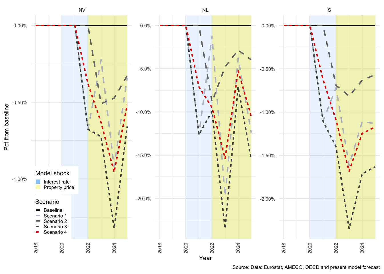
Figure 3.20: NFC Net Lending components

The major determinants of investment are therefore the major determinants of GDP, together with previous capital accumulation in NFC (previous capital, plus investment less depreciation). As can be seen in Figure , \(I^N\) (INV in the plot) is fist affected by Scenario 1 (interest rates) in 2022, this the change in NL observable is 2021 is purely due to the decline in savings. Although the shapes of the panels in Figure are very similar, the scales are quite different. The actual underlying values of each category are also significantly different. Plotted as actual values in Figure , the changes would be almost indiscernible from the baseline.

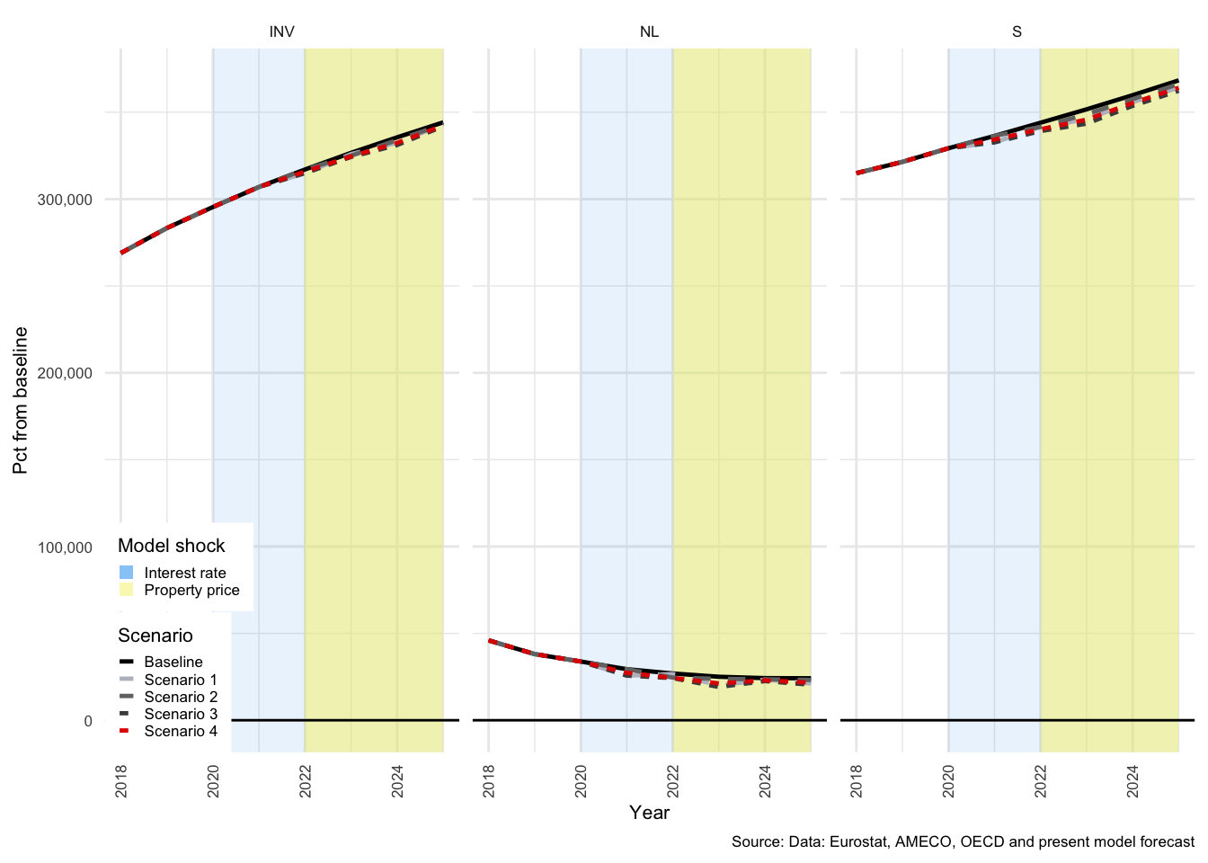
Figure 3.21: NFC Net Lending components

NFC savings (\(S^N_t\)), can be calculated as the net sum primary and secondary income and expenditures.

\[\begin{equation} \begin{split} S^N_t = & Y_t - WB^N_t + (B2^N_{t} - B2_{t}) + r^N_{t-1}(NIB^N_{t-1})\\ & + \chi _t (NEQ^N_{t-1}) - T^N_t + STR^N_t + \epsilon ^N \end{split} \end{equation}\]

\(NPIR-NEQ\) and \(STRA\) are exogenous, and revert to zero values after the last period of available data, 2017.

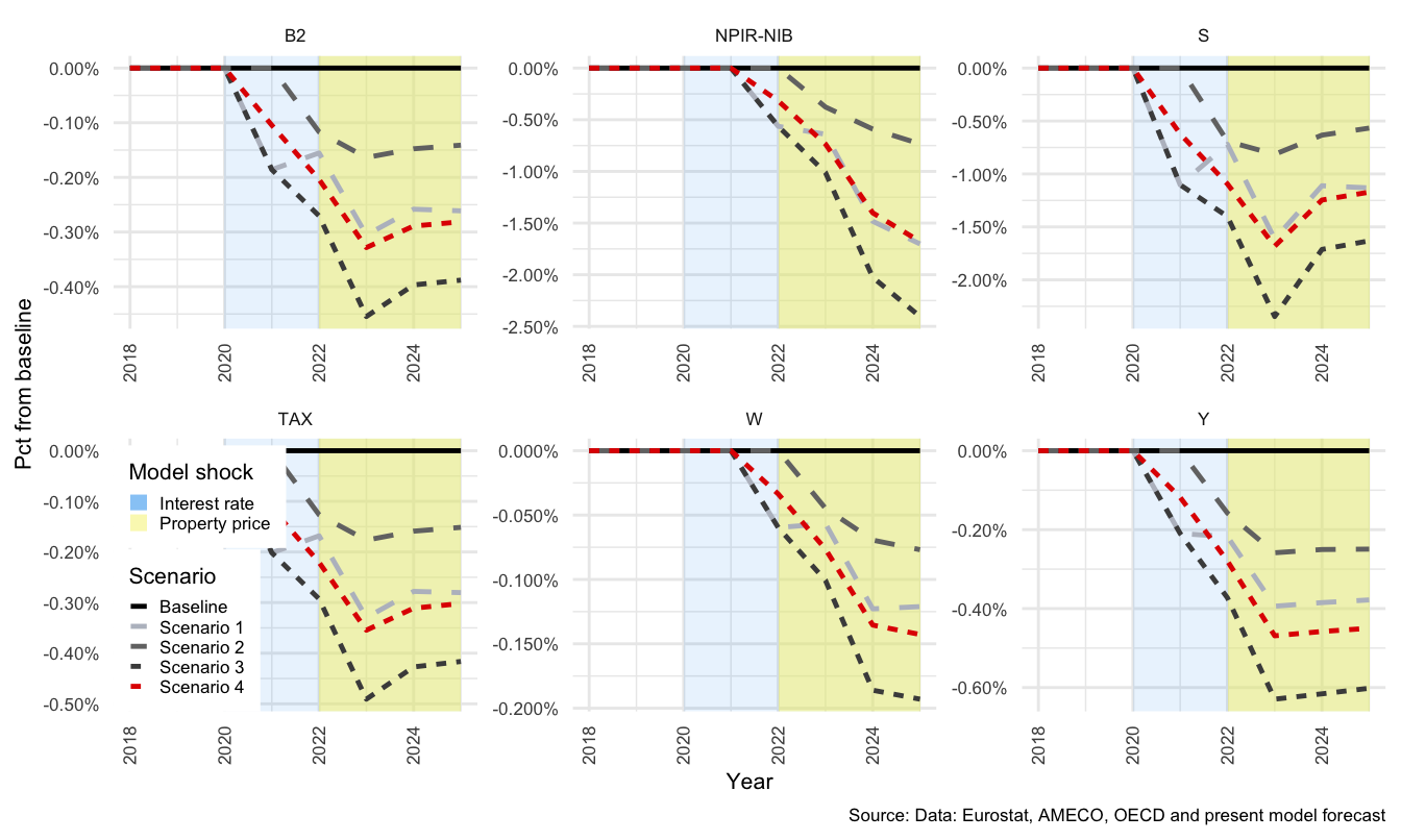
Figure 3.22: NFC Savings components

3.6.4 Effects for the GOV sector

For Scenario 1, in 2021 \(NIBTR^G\) is -30.78 % lower than the baseline. The source of this decline can be traced through the plots below. Figure shows the decline in net lending and savings.

Contributing to the decline in \(NL^G\) is a decline of -11.85% in \(S^G\). The main contributor to which is a fall in \(T^G\) of -1.56%. The net issue of \(IBL\) results in a fall in \(NIB^G\) of -9.16% and for net wealth to decline by -1.3%.

By 2023 the first shock has spread through the economy and \(NL\) is -34.27% below the baseline levels. The delayed effect of the change in interest rates is by that stage in effect, and results in a decline in net property income of -15.36%. This contributes to a reduced level of \(S^G\) of -14.07% below. The major contributor is a -1.47% lower level of tax revenue.

Social transfers for each sector, \(STRA^G\) in the case of GOV, are a net value of receipts less payments. \(STRA^G\) declines by -1.21%, indicating that the level of payments has increased relative to receipts. This contributes further to the negative balance in GOV. The decline in \(NIBTR^G\) above accumulates in \(NIB^G\) that is -19.27% lower than the baseline, and net wealth, \(NW^G\), that is -4.02% lower.

Shock 2 in 2022, the property price decline, has very little impact on GOV, with only a marginal decline in \(S^G\), flowing from limited impacts to the underlying components. \(NL^G\) falls by only -0.97%. This since tax revenues are only marginally affected when HH disposable income remains fairly constant, and the ultimate effect on \(NIB^G\) is only -0.24%. In reality this could have been substantially worse if the property price collapse resulted in non-performing loans and GOV was required to step in, as was the case for the banking crisis in Sweden in 1993. (Englund 1999)

By 2025, the effects remain modest, with \(NL^G\) only -1.93% down from the baseline level, and \(NW^G\) only -0.27% lower.

The largest changes in Scenario 1 for GOV in 2021 are in the residual financial flow for GOV, transactions in net interest bearing assets (\(NIBTR^G\)). These changes come almost entirely from changes in \(NL\), another term for which would be a government deficit or surplus, for negative and positive \(NL\) respectively. GOV issues debt (\(NIBTR^G\)) to cover the deficit. These assets are accumulated by FC (below), together with property income flows according to the return on these assets (\(r_N\)). As can be seen from Equation () below,

\[\begin{equation} NIBTR^G_t = NL^G_t \label{eq:nibtrg_intext} \end{equation}\]

Government investment (\(I^G\)), (and, as with NFC) \(NP^G\) and \(KTR^G\) are exogenous, so in Equation () below, it is only changes in savings (\(S^G\)) that are influential after the shocks in each scenario.

\[\begin{equation} NL^G_t = S^G_t - I^G_t - NP^G_t + KTR^G_t \label{eq:NL_G_intext} \end{equation}\]

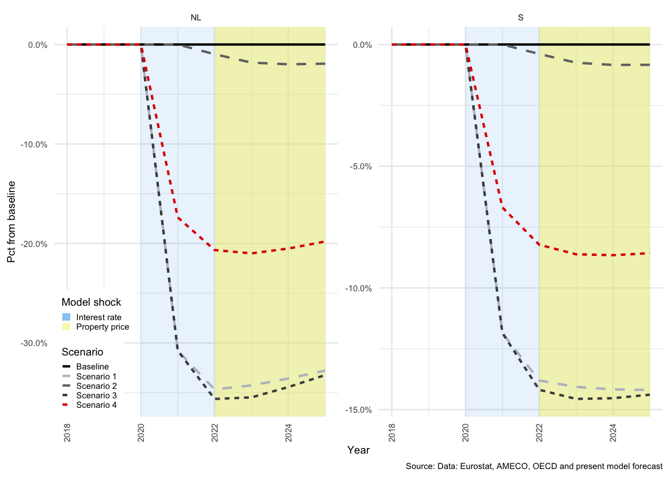
Figure 3.23: GOV Net Lending components

Equation () highlights the core components of GOV income. Of these \(B2^G\)+ net property income received, (\(r_{N_{t-1}}(NIB^G_{t-1})\), and NPIR in the plot below) and tax \(T^G\) are the incomes received by GOV. Social transfers (\(STR^G\), STRA in the plot below) and GOV expenditure (\(G\)). The exogenous component from the incomes is \(B2\), and from expenditure \(G\).

\[\begin{equation} S^G_t= B2^G_t + r_{N_{t-1}}(NIB^G_{t-1}) + T^G_t+ STR^G_t - G_t + \epsilon ^G \label{eq:savings_G_intext} \end{equation}\]

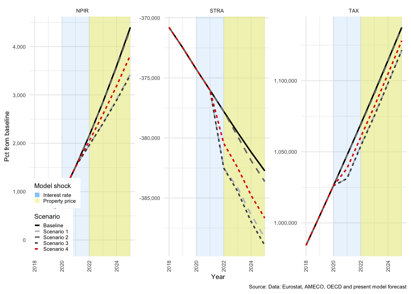
Figure 3.24: GOV Savings components

Considering Scenarios 3 and 4, the difference in the impact of shocks is about half as strong for Scenario 4, where \(\alpha\) is at 80%. Scenarios 1 and 3 however result in stronger effects. The impacts to GOV are directly a result of the deterioration in HH cash flows and needs for social support. While \(STR^G\) is the expenditure of GOV that flows to HH, based on total net benefit and contribution flows. Rising \(STR^G\) expenses are exacerbated by a fall in revenues in the form of both net property income received (NPIR) and taxation \(T^G\) (TAX in the plot above.)

3.6.5 Effects for the ROW sector

The ROW sector is primarily driven by exports, which are exogenous, and imports, which are endogenous to changes in the level of household income. The sharp decline in household income causes an immediate improvement in the current account balance, which is reflected as a negative NL balance for ROW³⁶.

For shock 1, in 2021, ROW is driven into a further deficit to Denmark, with a decline of -10.97% in \(NIBTR^W\), which captures the -10.97% decline in \(NL^W\) and \(S^W\). This has a negative effect of -0.7% on the level of net wealth (\(NW^W\)) held by ROW in Denmark.

The deficit in \(NL^W\) continues to grow, and by 2023 is -10.97% lower than the baseline value. The net flow of property income on all financial assets is lower by %, which reflects a -1.21% fall in the stock of \(NIB^W\). From a balance sheet perspective, there is a decline of -0.7% in net wealth (\(NW^W\)).

The second shock, to property prices has less of an impact on ROW, with \(NIBTR^W\) still lower, but in 2022, this is only by -8.14%. This is again driven by an equal decline in \(S^W\), which leads to an equal decline in \(NL^W\). The fall in \(NIBTR^W\) is reflected as a decline in \(NIB^W\) by -0.87%.

By 2025, the shock has spread through the economy, and the impact on \(S^W\), \(NL^W\) and \(NIBTR^W\) is lower again at -11.74% less than the baseline value. The changes in interest earning assets reduce the level of property income from \(NIB^W\) by -3.14%, and from all financial assets by -1.71%. The level of \(NIB^W\) continues to fall further into deficit by -3.98% relative to the baseline. After the three year period of accumulative effects, \(NW^W\) would be -2.69% lower.

The transmission of these shocks, working backwards from the accumulative effect on transactions in \(NIB^W\), begins with Equation ().

\[\begin{equation} NIBTR^W_t = NL^W_t - NEQTR^W_t - NPENTR^W_t \label{eq:NIBTR_row_intext} \end{equation}\]

Equation () describes the source of changes in \(NIBTR^W\), where \(NEQTR^W\) and \(NPENTR^W\) are exogenous in the model. This leaves only \(NL\) as a possible source of change. Unlike the domestic sectors, ROW is assumed not invest in the domestic economy, which means that the net lending function is somewhat simpler, with only savings as the possible source of change.

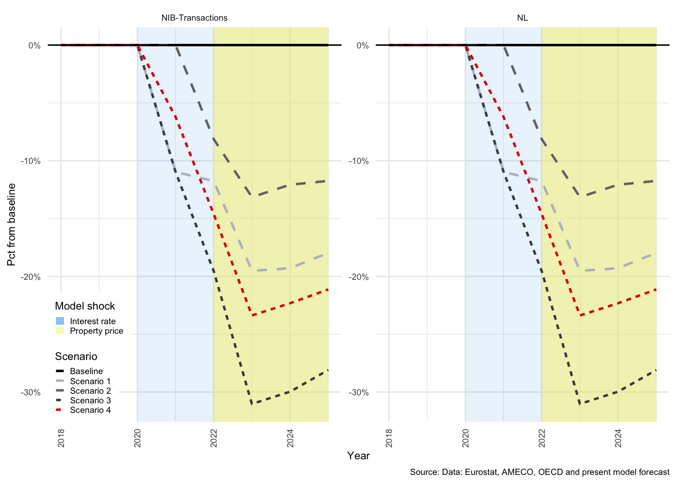
Figure 3.25: ROW: NIBTR: Transactions in assets and net lending

Equation () highlights the components of \(NL\), and much like the previous sectors, only \(S^W\) is endogenous in the model.

\[\begin{equation} NL^W_t = S^W_t - NP^W_t + KTR^W \label{eq:NL_row_intext} \end{equation}\]

It is therefore only savings that drives changes in \(NL\). The total level of \(NL\) is then, as mentioned earlier, equivalent to the current account balances - although what is positive in the current account must be negative in the ROW \(NL\) account.

\[\begin{equation} CAB_t = -NL^W_t \label{eq:CAB_row_intext} \end{equation}\]

Savings are described by Equation ().

\[\begin{equation} \begin{split} S^W_t = & M_t - X_t+\chi _t(NEQ^W_{t-1}) + \psi _t(NPEN^W{t-1}) + r_{N_{t-1}}(NIB^W_{t-1})\\ & + WB^W_t - T^W_t +STR^W_t +\epsilon ^W \label{eq:Savings_row_intext} \end{split} \end{equation}\]

ROW is assumed to be largely independent of developments in the domestic economy, and thus \(WB^W\), \(\chi _t(NEQ^W_{t-1})\), \(\psi _t(NPEN^W{t-1})\), \(STR^W\), and \(T^W\) are considered to be exogenous. This is with the exception that the rates of return on each of the asset classes is assumed to be the same as those available domestically. The reason for this is that Denmark is a AAA rated country and maintains a fixed exchange rate regime with the EU, and arbitrage keeps rates of return very close to those available in neighbouring Europe.

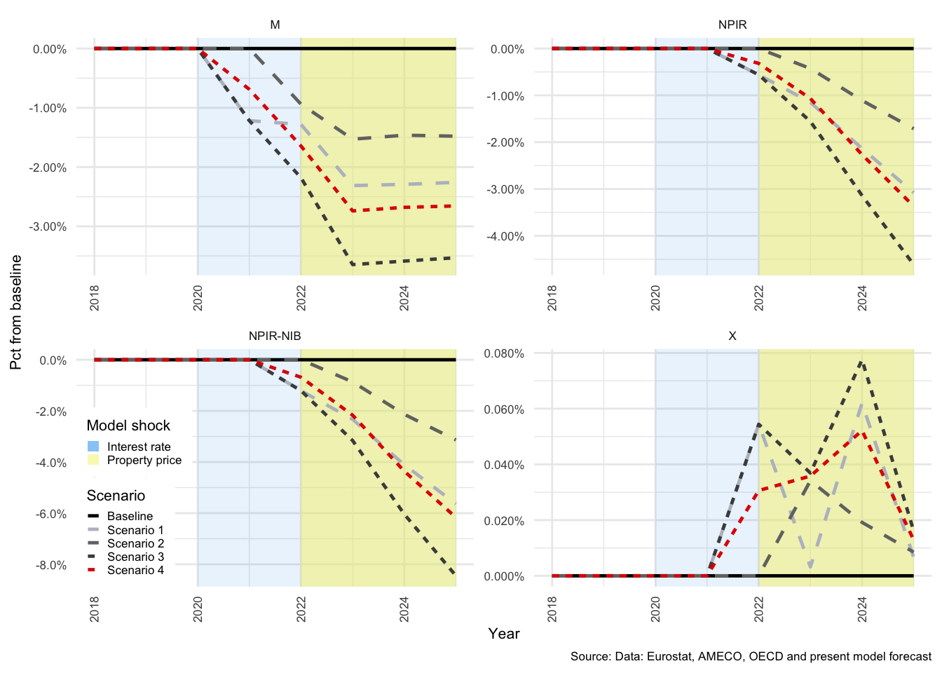
Figure 3.26: ROW Savings components

Imports (\(M\)) from the model are a revenue for ROW and exports (\(X\)) an expenditure. The return on net interest bearing stocks, \(r_{N_{t-1}}(NIB^W_{t-1})\), (NPIR-NIB in the plot above) depends on whether \(NIB^W\) is positive or negative.

Imports are estimated in real terms in the log-linear form in Equation (), and depend on the level of domestic demand in the previous period, and a relative price index between domestic and foreign goods from the previous period \(\Bigg( \frac{P^y_{t-1}}{P^m_{t-1}} \Bigg)\).

\[\begin{equation} ln(m_t) = \beta _i + \beta _iln \Bigg( \frac{P^y_{t-1}}{P^m_{t-1}} \Bigg) + \beta _iln(c_{t-1} + i_{t-1} + x_{t-1}) \label{eq:imports_intext} \end{equation}\]

As noted by Byrialsen and Raza (2019), the “export function is based on the Armington (1969) model where the market share of the Danish exports is explained by relative prices.”

This relation is captured below as annual Danish exports relative to a weighted index of all trading partners (\(m^W_t\)), which should be determined by domestic prices (the export price index, \(P^x_t\)) relative to foreign prices (the import price index, \(P^m_t\)), but moderated by price elasticity (\(\beta\)).

\[\begin{equation} \frac{x_t}{m^W_t} = \Bigg( \frac{P^x_t}{P^m_t}\Bigg)^ \beta \end{equation}\]

Exports thus stay relatively stable in the model, and are only affected by minor changes in the relative price ratio. The lower right panel in Figure above is a little deceptive, as the scale is very small. The most important change for ROW is a strong decline in Danish imports, which is primarily driven by the fall in HH disposable income

3.6.6 Effects for the FC sector

FC absorbs all of the imbalances in the other four sectors, and the relatively extreme shock to interest rates culminates in large changes to each. Transactions in net interest bearing assets, \(NIBTR^F\), are simply an inversion of the accumulation of \(NIBTR\) in three of the four sectors (GOV, NFC and ROW), and \(IBLTR^{F\sim H}\) is a reflection of household accumulation of deposits, \(IBATR^H\).

\[\begin{equation} NIBTR^F_t = -(NIBTR^N_t + NIBTR^G_t + NIBTR^W_t ) \label{eq:nibtr_f_intext} \end{equation}\]

The second, and rather indirect accumulation is that of equities to offset any equity investment by HH. The full explanation is available in the appendix, in Section . An abbreviated summary is that all other components of Equation () are accounted for by accounting identities between FC and the other sectors, and the value of \(EQATR^H\) is carried into FC via \(IBLTR^{F\sim H}\). Once all other terms are netted out, the \(NEQTR^F\) value is equivalent to \(EQATR^H\). This equivalence is the redundant equation in the model, and is not specified in order to avoid over-identification.

\[\begin{equation} NEQTR^F_t = NL^F_t + IBLTR^{F\sim H}_t + PENLTR^F_t - IBATR^{F\sim H}_t - NIBTR^F_t \label{eq:neqtr_fc_intext} \end{equation}\]

Because \(NIBTR^F\) captures the net flows of all other sectors, it also represents any excess or shortfall (i.e. net lending) experienced by FC. This is because all flows of all other sectors with each other will already be captured and netted out by the sum of their \(NIBTR\) in Equation () above. The only unaccounted for flow is the net value of FC flows, which is captured in \(NL^F\). Again, \(NP^F\), \(I^F\)³⁷ and \(KTR^F\) are exogenous.

\[\begin{equation} NL^F_t = S^F_t - I^F_t - NP^F_t + KTR^F_t \end{equation}\]

Rather than show the percentage changes, Figure shows the actual increase in FC NL and savings as a result of the shocks in each scenario. As can be seen, the impact of the second shock is almost negligible. Scenarios 1 and 3 are almost identical, and Scenario 2 remains very close to the baseline level. It is thus the interest rate change that has the dominating effect on FC’s flows and thus balance sheet. It should be unsurprising therefore that there is a substantial difference between Scenarios 3 and 4. In Scenario 4, where a greater portion of HH debt is less sensitive to changes in interest rates, the transfer of wealth from HH to FC is substantially reduced.

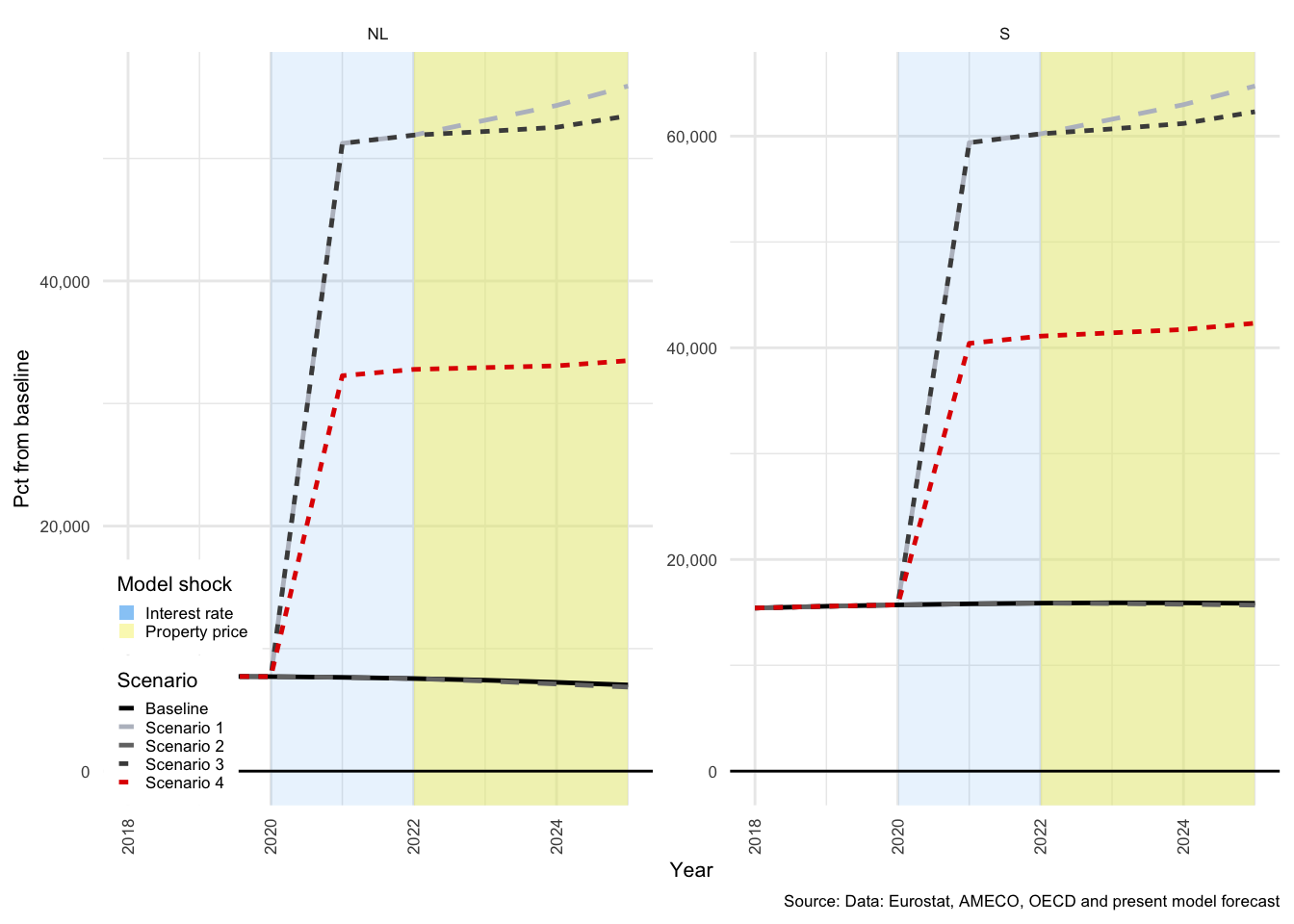
Figure 3.27: FC Net Lending components

From a very low base, \(NL^F\) rises by 569.17%, or is roughly five and a half times larger. The shifts in the values of the underlying FC components are sensibly also substantial. Transactions in most assets are net positive, and in liabilities negative - both relative to the baseline and in absolute terms.

The exception is a decline in loan assets as HH deleverage in 2021 by -3.23%. Apart from this single entry, HH borrowing is positive in all periods. Relative to the baseline after the first shock, \(IBLTR^{F\sim H}\) is down by -78.28%, and \(IBATR^{F\sim H}\) is down by -73.94%. FC is a net issuer of equity and interest bearing assets, with transactions in equity, \(NEQTR^F\), up 68.34%, and in \(NIB\) up 61.82%. FC thus begins to accumulate assets rapidly.

In terms of property income flows, the rise in interest rates in this example is only allowed to affect the asset returns of FC, and thus the net increase is more extreme than if we adjusted all rates of return. The total net property income received by FC, \(NPIR^F\), is 323.58% higher. This comes from the increase in fixed and flexible rate interest receipts, which rise by 32.38%, and 136.29% respectively.

As noted above, FC accumulates assets rapidly. \(NEQ^F\) rises by 46.26% and \(NIB^F\) by 2.02%. The fall in \(IBA^{F\sim H}\) by -2.26% and in \(IBL^{F\sim H}\) by -3.23% almost offset each other entirely, and the final impact on net wealth of FC is an increase of 42.82%.

Equation () highlights the income and expenditure components that contribute to FC savings, and Figure illustrates these components in nominal values.

\[\begin{equation} \begin{split} S^F_t = & B2^F_t \\ & + r^F_{A(FI)_{t-1}}(IBA^{F\sim H}_{A(FI)_{t-1}}) + r^F_{A(FL)_{t-1}}(IBA^{F\sim H}_{A(FL)_{t-1}}) \\ & - r^F_{L_{t-1}}(IBL^{F\sim H}_{L_{t-1}}) + r_{N_{t-1}}(NIB^F_{t-1}) \\ & + \chi _t(NEQ^F_{t-1}) -\psi _t(PENL^F_{t-1}) - T^F_t + STR^F_t - CPEN^F_t + \epsilon ^F \end{split} \label{eq:S_fc_intext} \end{equation}\]

From Equation (), \(B2^F\) and \(T^F\) are exogenous, and the change in FC output, \(Y^F\), is less than -1%. Nominal values are illustrated here in order to give better context to the changes implied by the shocks. The percentage changes that are discussed above for Scenario 1 do not appear to be as unrealistic when viewed in these terms.

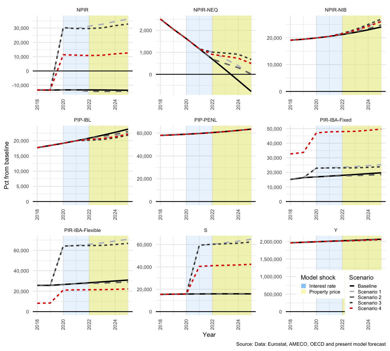
Figure 3.28: FC Savings components

The panel titled net property income (NPIR) in the plot above is a sum of all property income flows, and is similar to Equation () above for \(S^F\), but with all other terms removed. The total impact on property income helps to identify the source of changes in FC savings. NPIR is calculated as follows.

\[\begin{equation} \begin{split} NPIR^F_t = & + r^F_{A(FI)_{t-1}}(IBA^{F\sim H}_{A(FI)_{t-1}}) + r^F_{A(FL)_{t-1}}(IBA^{F\sim H}_{A(FL)_{t-1}}) \\ & + r_{N_{t-1}}(NIB^F_{t-1}) + \chi _t(NEQ^F_{t-1}) \\ & -\psi _t(PENL^F_{t-1}) - r^F_{L_{t-1}}(IBL^{F\sim H}_{L_{t-1}}) \end{split} \label{eq:NPIR_fc_intext} \end{equation}\]

The bulk of FC flows are property income paid (PIP), property income received (PIR), or NPIR. The representations in Figure above are categories of these property income flows. NPIR-NEQ for \(\chi _t(NEQ^F_{t-1})\) (on equities), NPIR-NIB for \(r_{N_{t-1}}(NIB^F_{t-1})\) (on net interest bearing assets with all sectors other than HH), PIR-IBA-Fixed for \(r^F_{A(FI)_{t-1}}(IBA^{F\sim H}_{A(FI)_{t-1}})\) (on fixed-rate HH debt), PIR-IBA-Flexible for \(r^F_{A(FL)_{t-1}}(IBA^{F\sim H}_{A(FL)_{t-1}})\) (on flexible-rate HH debt), PIP-IBL for \(r^F_{L_{t-1}}(IBL^{F\sim H}_{L_{t-1}})\) (on deposit liabilities).

The shock to interest rates in Scenarios 1, 3 and 4 all result in positive NPIR for FC. The substantially lower level of NPIR in Scenario 4 (the red line) can be traced back to PIR-IBA-Fixed and PIR-IBA-Flexible. The sum of the total revenue generated by the rise in interest rates is the summarised in NPIR. The steady decline of net return on equities, NPIR-NEQ, is due to the systematic issuance of equity to HH as HH demands equity. This demand is retarded slightly in all scenarios. Equity investment by HH is dependent on previous returns, previous returns on house investment and previous changes in the quantity of loans acquired. For both shock 1 and 2, it is due to the reduction in \(IBLTR^H\) and for shock 2 it is also driven by a fall in returns on houses.

The effect on FC savings, \(S^F\), is to triple the value in Scenarios 1 and 3, and double the value in Scenario 4.

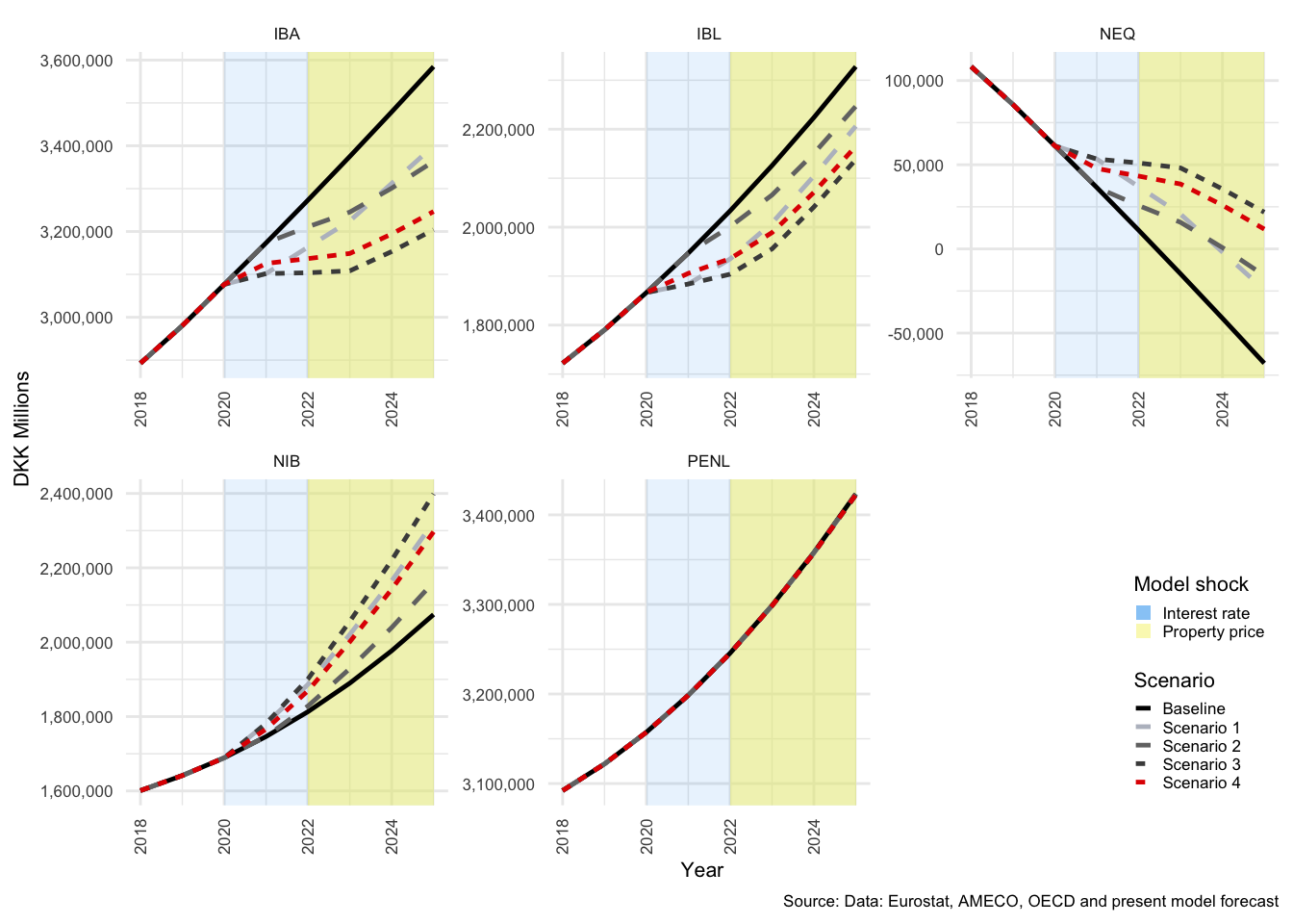
Figure 3.29: FC balance sheet

3.7 Discussion

As noted in Section , many of the innovations that occurred around the world during the past decades also occurred in the Danish mortgage lending system. In addition, since the GFC, interest rates have reduced to and remained at historically low levels. These conditions provided the platform for rapid expansion of household mortgage debt leading up to the crisis, and to continued expansion of that debt in more recent years. This has coincided with the rapid recovery and inflation of asset prices. Property prices are discussed in Section above, and as can be seen from panel (a) in Figure , Danish equity prices (the yellow line) have risen over 230% from 2010 to 2018, with only one other European country (Latvia, the blue line) with a higher increase in its equity price index.

The main effects of the innovations that occurred were a reduction in initial payments for borrowers, a decline in the level of payments towards the outstanding principal debt (and thus a decline in the level of equity accumulation) and a significant shift of risk from investors to lenders. Danish HH responded rapidly to the innovations, and the composition of debt changed from 100% fixed interest debt, in 2000 to less than 30% by 2012, as can be seen in panel (b) of Figure ³⁸.

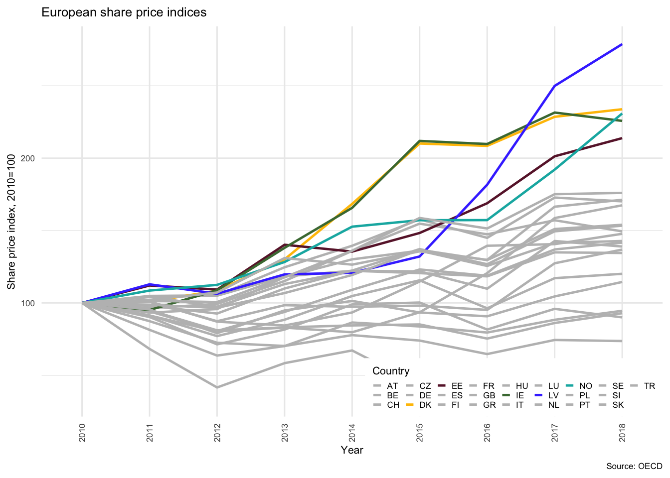
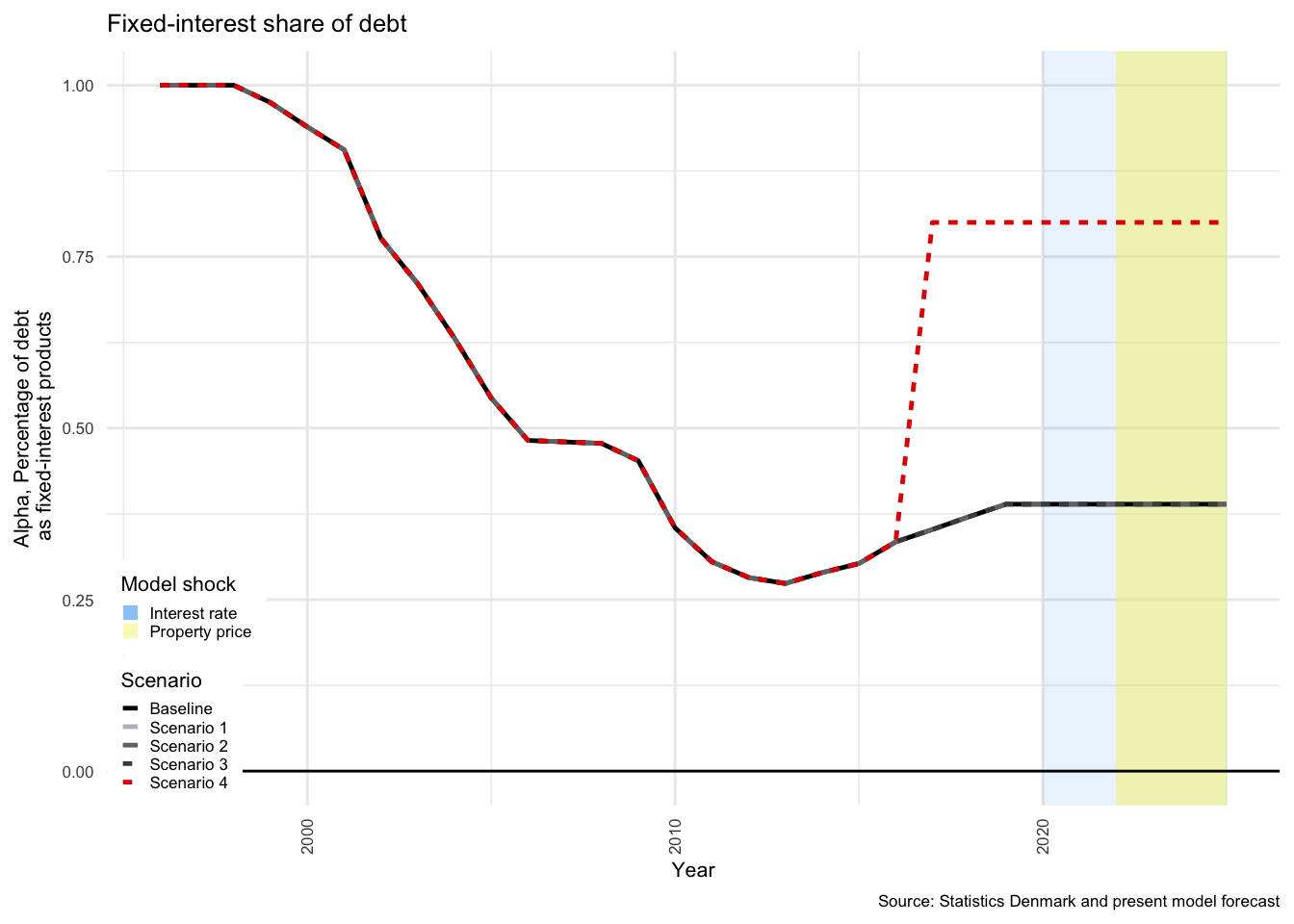
Figure 3.30: Share prices and mortgage composition

The major benefits of fixed interest products include stability of expenditures, insulation against unforseen interest rate hikes, and the possibility to refinance at various favourable instances (stemming from the buy-back, and prepayment rights assigned to borrowers (Skinhøj et al. 2019)). Flexible interest rate products on the other hand, provide low initial cost of borrowing, but transfer interest rate risk to the borrower. Revisions to the coupon rate on the counter-balancing bonds also create a significant opportunity cost for ARM borrowers if rates rise. This is opportunity cost is enhanced if it is a distressed borrower, or the borrower faces negative shocks, such as a loss of income or an injury. A fixed rate borrower (even without amortization) would be able to accept a lower sale value for their property, since the bond that represents the outstanding debt would reprice downwards as interest rates rise. In the case of an interest rate increase, flexible rate borrowers face the same possibility of unfavourable property market conditions, but the price of bonds outstanding will remain relatively constant, due to the re-setting of the short-term fixation of coupon payments. Flexible rate borrowers, and borrowers with interest-only periods thus face a much higher risk of falling into negative equity if house prices fall.

Many of these dynamics are captured in the model presented in this article, as are several economic relationships between the real and financial sides of the economy. These connections make it possible to show some of the expected “real” economic feedback effects of each shock. Although it is a highly simplified version of the Danish mortgage market, it is still able to provide a realistic scale for the core transmission channels for each of the shocks, and due to the simple structure of the model, it was relatively easy to incorporate a split in the composition of debt of HH.

One of the goals at the outset was to test the sensitivity of HH balance sheets for different compositions of debt. Two shocks were introduced across four scenarios. The primary effect of the first shock, an increase in interest rates by 2% in 2020, was an immediate reduction in HH income. The primary effect of the second shock, a decline in property prices by 20% in 2022, was to reduce the level of HH capital and the attractiveness of housing as an investment alternative. These two shocks were then compounded in Scenarios 3 and 4, but in Scenario 4 the level of debt held in fixed-interest products (\(\alpha\)) was increased from around 37% to 80%, as shown in panel (b) of Figure above.

The model behaved as expected, and in Scenario 3, with the higher proportion of ARMs, HH are exposed to significantly greater income volatility than in Scenario 4, a result that is corroborated by Danmarks Nationalbank (2016) and Skinhøj et al. (2019). This transmits to both the real and financial sides of the economy, with lower economic output and higher unemployment as a result of the increased sensitivity. The results in Section above suggest that for a significant rise in interest rates, or a collapse in property prices, HH would be in a more favourable financial position as a sector if the proportion of mortgage debt held in fixed-interest products (\(\alpha\)) was higher. This suggests that policies with a focus on increasing the coverage of fixed-interest-rate products in the mortgage financing system would result in a more resilient HH, and economy as a whole.

The specific movements of variables, however, should be interpreted with caution, as the shocks in this model are not designed to provide a comprehensive economic response within the model structure. Especially since it is only the rates that affect the cost of borrowing that are adjusted in shock 1.

In terms of the transmission channels in the model, HH is a key driver. The primary transmission channel in the interest rate shock is the credit channel, and it is clearly more impactful where interest rates are more sensitive. In a more realistic setting, the rise in interest rates would also affect HH incomes positively. In Denmark, pension funds hold a large portion of the outstanding covered covered bonds on behalf of households, and fees of the mortgage lending companies are generally a fixed rate. This would mean that increased mortgage costs should translate directly to increased pension incomes. HH pension assets are also substantially larger than HH debt, which means that if an interest rate hike resulted in a rise of the rates of return on most asset classes, then HH could experience a net gain. One argument against this is that pension assets are not directly accessible, and therefore would not contribute to short term disposable income of HH. HH in this case do not have discretion over the consumption of all wealth, and therefore those parts that are inaccessible should be excluded.

The current form of the model is also important to consider. Presently, HH consume out of wealth, and there is a positive return on \(IBA\), which are assumed to be deposits. If we adjust the rate of return on \(IBA\) (\(r^H_N\)) upwards, it would change relative rates of return available for HH investment allocation, and would lead to a rapid accumulation of \(IBA\). It would also drive a large positive effect on HH income, which would conceal the negative effects to disposable income that are displayed in the current form. This would, at least in the short run, not be in line with realistic expectations regarding accessible disposable income of HH.

Even if other asset class returns are adjusted to mitigate the fall in HH disposable income, investment will necessarily be lower as the cost of borrowing rises. In the case of an interest rate rise, aggregate demand and output would still decline, pushing unemployment upwards and providing downward pressure on the wage rate. after several years, the relative improvement in competitiveness in export prices would have a positive influence on exports and negative on imports. Ultimately this would strengthen the current account balance, but at the expense of higher unemployment in the domestic economy. The positive feedback of rising imports on wage income and output would depend on the elasticities of wages to changes in output, and imports and exports to relative price changes. The effect of a fall in house prices on housing investment would also remain in the short-term, as it is dependent on previous returns.

Another transmission channel that would be concealed is the negative pressure that a fall in demand has on the tax base, and therefore on GOV revenues. In the analysis above, it is clear that the fall in overall demand would lead to a fall in employment, a fall in tax revenues and therefore a large negative shift in the GOV net financing requirement. If the Danish GOV enforces a balanced budget, there would need to be a reduction in GOV spending, and the vast majority of this spending is split between a tax funded pension scheme, healthcare, disability support, family and child support. A reduction in any of these categories would result in a further reduction of output and ultimately in HH income.

Even with the simplifications, it should be safe to conclude that larger portions of debt in fixed-interest products would result in much lower volatility of HH disposable income. The use of a more comprehensive model, rather than a simple test of income volatility, allows us to observe the expected accumulation effects of the two shocks for different levels of \(\alpha\). The exogeneity of asset prices and rates of return are potential drawbacks, however, it is not obvious that creating endogenous links between financial markets, assets and rates of return (i.e. a more integrated financial sector) would be an improvement on the current model structure. At present, the most immediate transmission channels for each of the shocks are transparent, and because of the empirical nature of the model, it is possible to get an accurate scale of the initial effects of the shocks, without the complication of complex interdependencies between markets. There is a clear trade-off between complexity with greater accuracy, and better interpretability with greater transparency.

The more complete macroeconomic SFC model presented above requires attention to the gross levels of economic stocks and flows, and thus makes it possible to identify that the rise in HH \(NL\) following the second shock (the fall in property prices) was not due to positive changes in HH. Contrarily, HH experienced a decline in investment demand, together with rising unemployment. The model presented here helps to prevent such misinterpretations, and to provide a more complete picture of the possible impact of shocks³⁹.

The model unfortunately does not presently incorporate some key issues from the mortgage system, including the effect of changes in loan-to-value (LTV) ratios, or second round credit risk effects that might occur due to loss of income due to unemployment. The inclusion of a measure of non-performing loans or some other measure of credit risk might be able to capture these effects. Perhaps the most relevant omission, for the present discussion, is the effect of refinancing behaviour on the composition of debt, although this is not a simple matter to include, as noted by Skinhøj et al. (2019, 19), “The stochastic modelling of prepayment behaviour is a complex task and is outside the scope for most international investors.”

The possibility to explore a variety of modifications and alterations is also one of the major benefits that the baseline version of the model offers. It has made it possible to explore some of the complex economic feedback mechanisms described above. This version is also under continuous development by the MaMTEP group⁴⁰, and as additional economic components are explored in greater detail it will be possible to include any alterations that strengthen the core structure.

3.8 Conclusion

The Danish mortgage financing system has experienced several innovations in recent decades. Collectively these innovations have had a variety of benefits for borrowers, but these come with a transfer of responsibility and risk to the borrower. One of the most prominent innovations was the introduction of adjustable rate mortgages (ARMs) with periods of interest fixation of a variety of lengths.

Access to individual level administrative data-sets allowed for the construction of aggregate outstanding mortgage data from 2009 to 2017, and highlights the increased concentration of flexible-rate mortgage debt. By the end of 2017, after the introduction of ARM products, approximately 63% of all mortgage debt outstanding was subject to an interest rate adjustment within 5 years. These products were collectively considered to be flexible-interest rate products in the analysis above, and the remaining debt considered to be fixed rate.

The model in this article was adapted from Byrialsen and Raza (2019) to explore the effects of this shift on the stability of incomes and balance sheets of the Danish economy. The primary innovation in the model was to introduce the split in debt, and to test the effect of the changes on the overall sensitivity of incomes and balance sheets, with a particular focus on HH. There are some additional changes that could be incorporated in future versions of the model that might strengthen the outputs of the model. Firstly, additional data could be sourced to provide a further split in HH debt between mortgage institute, bank and consumer debt. Secondly, it might be possible to actively model the refinancing behaviour of Danish property buyers⁴¹. It might also be possible to include some measure of credit supply constraints, and or borrower risk, for example, non-performing loans. Further developments of the model could make this possible.

The core aim of the analysis was to test the sensitivity of HH and economic conditions of a potential shift in the composition of debt from ARM type products to fixed-interest products. This is an intuitively simple proposition, but the accurately scaled empirical model presented in this article provides a clear indication of the potential scale of these impacts. For a shift in the fixed proportion from 37% up to 80%, in the case of a 2% point increase in interest rates and a 20% decline in property prices, the difference in aggregate unemployment effects could be as much as 2%. The effects discussed for each sector mirror this increase in sensitivity. Both in the initial effects and in terms of volatility in subsequent periods.

The results thus provide evidence to support reports made by the IMF (Sheehy 2014), the Danish national bank (Danmarks Nationalbank 2016) and the leading mortgage credit institution in Denmark, Nykredit Realkredit (Skinhøj et al. 2019), that the increased concentration of household debt in ARM (flexible-rate) products has resulted in greater sensitivity (and thus less stability) of both HH and the Danish economy in general. This does not imply that the level of outstanding debt poses a systemic economic risk. Again in support of reports presented by the above institutions, it should be noted that simultaneous and sizable shocks to both the cost of borrowing and to property prices only resulted in modest effects on overall output, even where the shock is restricted to borrowing costs.

In contrast to suggestions regarding the systemic risk of household debt in itself, the analysis suggests that the potential risks related to the present high ratio of HH debt to disposable income in Denmark can be dramatically reduced through a migration of HH mortgage debt away from ARM type products towards fixed interest rate products. The all-time low levels of interest rates that are currently available also present an excellent opportunity to support this transition.

3.9 Appendix

3.9.1 Mortgage debt as a percentage of total loans to non-financial private sector (nominal, local currency)

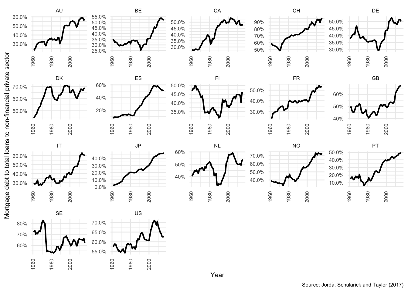
Figure 3.31: Mortgage debt as percentage of total loans

3.9.2 Mortgage debt to GDP

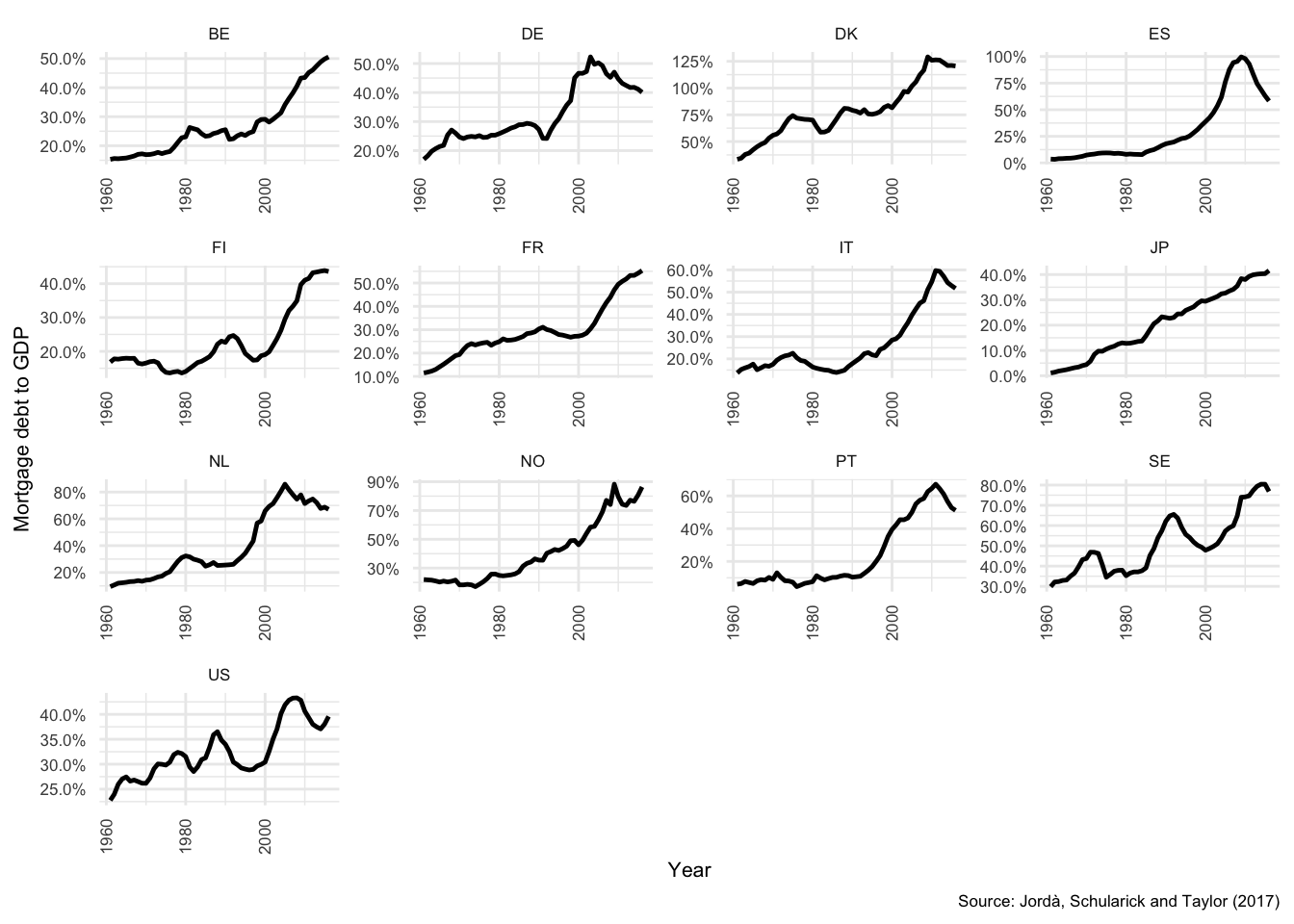
Figure 3.32: Mortgage debt to GDP

3.9.3 House Prices

Table 3.4: OECD House price index changes, Year on year

Country	2000 to 2007	2007 to 2009	2009 to 2018
Estonia	15.89%	-17.06%	11.33%
Costa Rica	08.94%	06.07%	04.11%
Austria	03.63%	03.01%	03.97%
Colombia	04.58%	04.79%	03.85%
Hungary	13.52%	08.14%	03.01%
Czech Republic	05.25%	16.46%	02.83%
United States	04.10%	01.82%	02.78%
Netherlands	03.35%	02.03%	02.62%
Ireland	16.65%	-12.57%	02.50%
Finland	02.96%	00.33%	02.43%
Israel	00.55%	05.02%	02.40%
Korea, Republic of	03.01%	01.93%	02.39%
Norway	03.72%	03.27%	02.35%
Poland	08.40%	05.06%	02.23%
Mexico	06.03%	03.23%	02.15%
New Zealand	00.97%	02.29%	02.07%
Denmark	03.11%	02.95%	01.98%
United Kingdom	03.52%	02.65%	01.95%
Portugal	03.37%	02.90%	01.76%
Sweden	02.56%	02.92%	01.56%
Latvia	11.22%	03.58%	01.39%
Luxembourg	02.87%	02.79%	01.31%
Germany	01.30%	01.17%	01.23%
Canada	01.64%	01.63%	01.09%
Slovenia	12.31%	02.53%	01.00%
France	03.36%	02.15%	00.82%
Italy	03.07%	02.95%	00.80%
Switzerland	01.87%	02.46%	00.75%
Slovakia	22.41%	04.09%	00.42%
Spain	05.69%	03.72%	00.29%
Greece	06.25%	03.82%	-2.33%
Japan	-0.27%	-0.22%	-0.31%

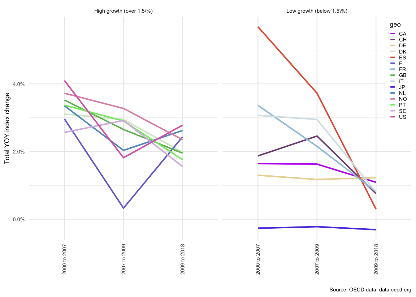
Figure 3.33: OECD house prices: Year-on-year changes

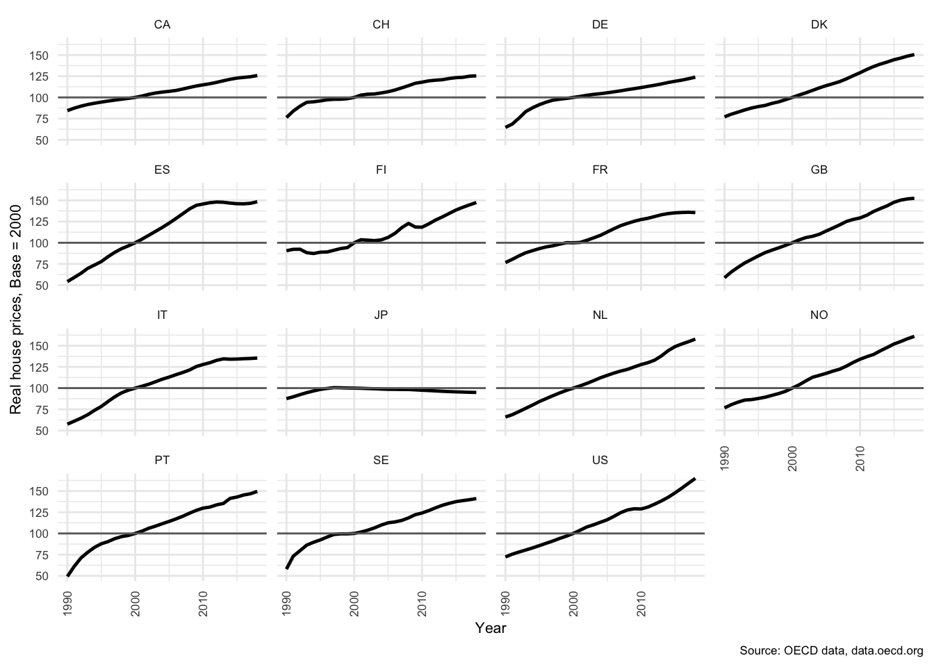
Figure 3.34: OECD house prices: Real price index

3.9.4 Simulation most affected variables in each shock

3.9.4.1 Scenario 1: Percentage from baseline: An increase in 2020 interest rates, measured in 2021

Table 3.5: Most affected variables: Perc change from baseline: Scenario 1, 2021: Economy wide

Variables	Type	Description	Change
PY	Deflation index	Price deflator: GDP	00.0082%
CAB	Flow	Current account balance	10.9700%
FAB	Flow	Financial account balance	-10.9700%
NX	Flow	Net Exports	10.5161%
I-Real prices	Flow	Gross fixed capital formation	-1.2468%
I	Flow	Gross fixed capital formation	-1.2468%
M	Flow	Imports	-1.2173%
M-Real prices	Flow	Imports	-1.2173%
PRIVATE	Flow	Gross income	-0.6908%
S-Real prices	Flow	Savings	-0.5725%
S	Flow	Savings	-0.5638%
Y-Real prices	Flow	Total income	-0.2097%
Y	Flow	Total income	-0.2016%
B2	Flow	Gross operating surplus	-0.1126%
ULC	Rate	Labour force: Unit labour cost: Price index: Index for the price deflator with reference to 2010 (all other price deflator indices are referenced to 2010)	00.2021%
UL-COST	Rate	Labour force: Unit labour cost	00.2020%
CU	Ratio	Capacity Utilisation (Real GNI / real capital stock)	-0.2098%
WS	Ratio	Wage share	00.0442%

Table 3.6: Most affected variables: Perc change from baseline: Scenario 1, 2021: HH

Variables	Type	Description	Change
PIP-IBL-HH-Flexible	Flow	Property income paid: IBL	136.2914%
PIP-IBL-HH	Flow	Property income paid: IBL	95.8530%
IBA-HH-Transactions	Flow	Financial Assets: Interest bearing assets	-78.2793%
FL-HH-Transactions	Flow	Financial liabilities	-73.9372%
IBL-HH-Transactions	Flow	Financial Liabilities: Interest bearing liabilities	-73.9372%
EQA-HH-Transactions	Flow	Financial Assets: Equity assets	-68.3376%
NPIR-HH	Flow	Net property income received: Total	-58.6600%
FA-HH-Transactions	Flow	Financial Assets	-54.5574%
PIP-IBL-HH-Fixed	Flow	Property income paid: IBL	32.3802%
FNL-HH	Flow	Financial Net Lending (Balance)	-16.6354%
NL-HH	Flow	Sector Balance	-16.6354%
S-HH	Flow	Savings	-10.3028%
INV-HH-Real prices	Flow	Gross fixed capital formation	-6.8066%
INV-HH	Flow	Gross fixed capital formation	-6.8066%
PIR-IBA-HH	Flow	Property income received: IBA	-3.2347%
Y-D-HH	Flow	Disposable Income	-2.5806%
Y-HH	Flow	Total income	-2.5806%
TAX-HH	Flow	Tax	-2.5806%
Y-D-HH-Real prices	Flow	Disposable Income	-2.5806%
C-HH-Real prices	Flow	Consumption	-1.3327%
C-HH	Flow	Consumption	-1.3326%
R-IBL-HH-Flexible	Rate	Rate of interest: Interest bearing liabilities	141.7474%
R-IBL-HH-Fixed	Rate	Rate of interest: Interest bearing liabilities	35.4369%
IBA-HH	Stock	Financial Assets: Interest bearing assets	-3.2347%
IBL-HH	Stock	Financial Liabilities: Interest bearing liabilities	-2.2569%
IBL-HH-Fixed	Stock	Financial Liabilities: Interest bearing liabilities	-2.2569%
IBL-HH-Flexible	Stock	Financial Liabilities: Interest bearing liabilities	-2.2569%
FA-HH	Stock	Financial Assets	-1.1087%
EQA-HH	Stock	Financial Assets: Equity assets	-0.8157%
K-HH	Stock	Stock of Capital	-0.2520%
K-HH-Real prices	Stock	Stock of Capital	-0.2520%
NW-HH	Stock	Net Wealth	-0.2223%
NW-HH-Real prices	Stock	Net Wealth	-0.2222%
FNW-HH-Real prices	Stock	Financial net wealth	-0.2044%
FNW-HH	Stock	Financial net wealth	-0.2044%

Table 3.7: Most affected variables: Perc change from baseline: Scenario 1, 2021: NFC

Variables	Type	Description	Change
FNL-NFC	Flow	Financial Net Lending (Balance)	-12.6166%
NIB-NFC-Transactions	Flow	Net financial stock: Interest bearing	-12.6166%
NL-NFC	Flow	Sector Balance	-12.6166%
S-NFC	Flow	Savings	-1.1026%
TAX-NFC	Flow	Tax	-0.2016%
B2-NFC	Flow	Gross operating surplus	-0.1858%
NIB-NFC	Stock	Net financial stock: Interest bearing	-0.5636%
NW-NFC	Stock	Net Wealth	-0.2341%
FNW-NFC	Stock	Financial net wealth	-0.2042%

Table 3.8: Most affected variables: Perc change from baseline: Scenario 1, 2021: FC

Variables	Type	Description	Change
FNL-FC	Flow	Financial Net Lending (Balance)	569.1674%
NL-FC	Flow	Sector Balance	569.1674%
NPIR-FC	Flow	Net property income received: Total	323.5769%
S-FC	Flow	Savings	275.5754%
PIR-IBA-FC-HH-Flexible	Flow	Property income received: IBA	136.2914%
IBL-FC-HH-Transactions	Flow	Financial Liabilities: Interest bearing liabilities	-78.2793%
IBA-FC-HH-Transactions	Flow	Financial Assets: Interest bearing assets	-73.9372%
NEQ-FC-Transactions	Flow	Net financial stock: Equity	68.3376%
NIB-FC-Transactions	Flow	Net financial stock: Interest bearing	61.8225%
PIR-IBA-FC-HH-Fixed	Flow	Property income received: IBA	32.3802%
Y-FC	Flow	Total income	-0.0442%
NEQ-FC	Stock	Net financial stock: Equity	46.2640%
NW-FC	Stock	Net Wealth	42.8191%
FNW-FC	Stock	Financial net wealth	23.0242%
IBL-FC-HH	Stock	Financial Liabilities: Interest bearing liabilities	-3.2347%
IBA-FC-HH	Stock	Financial Assets: Interest bearing assets	-2.2569%
NIB-FC	Stock	Net financial stock: Interest bearing	02.0236%

Table 3.9: Most affected variables: Perc change from baseline: Scenario 1, 2021: GOV

Variables	Type	Description	Change
FNL-GOV	Flow	Financial Net Lending (Balance)	-30.7775%
NIB-GOV-Transactions	Flow	Net financial stock: Interest bearing	-30.7775%
NL-GOV	Flow	Sector Balance	-30.7775%
S-GOV	Flow	Savings	-11.8501%
TAX-GOV	Flow	Tax	-1.5577%
FNW-GOV	Stock	Financial net wealth	-9.1649%
NIB-GOV	Stock	Net financial stock: Interest bearing	-9.1649%
NW-GOV	Stock	Net Wealth	-1.2954%

Table 3.10: Most affected variables: Perc change from baseline: Scenario 1, 2021: ROW

Variables	Type	Description	Change
FNL-ROW	Flow	Financial Net Lending (Balance)	-10.9700%
NIB-ROW-Transactions	Flow	Net financial stock: Interest bearing	-10.9700%
NL-ROW	Flow	Sector Balance	-10.9700%
S-ROW	Flow	Savings	-10.9700%
NIB-ROW	Stock	Net financial stock: Interest bearing	-1.2091%
FNW-ROW	Stock	Financial net wealth	-0.6953%
NW-ROW	Stock	Net Wealth	-0.6953%

3.9.4.2 Scenario 1: Percentage from baseline: An increase in 2020 interest rates, measured in 2023

Table 3.11: Most affected variables: Perc change from baseline: Scenario 1: Economy wide, 2023

Variables	Type	Description	Change
PY	Deflation index	Price deflator: GDP	00.0645%
PX	Deflation index	Price deflator: Exports	00.0293%
CAB	Flow	Current account balance	19.5257%
FAB	Flow	Financial account balance	-19.5257%
NX	Flow	Net Exports	18.9600%
I-Real prices	Flow	Gross fixed capital formation	-2.3220%
I	Flow	Gross fixed capital formation	-2.3220%
M-Real prices	Flow	Imports	-2.3121%
M	Flow	Imports	-2.3120%
PRIVATE	Flow	Gross income	-1.3215%
S-Real prices	Flow	Savings	-1.0950%
S	Flow	Savings	-1.0518%
Y-Real prices	Flow	Total income	-0.3939%
Y	Flow	Total income	-0.3297%
B2	Flow	Gross operating surplus	-0.1848%
X-Real prices	Flow	Exports	-0.0261%
X	Flow	Exports	00.0032%
UL-COST	Rate	Labour force: Unit labour cost	00.2739%
ULC	Rate	Labour force: Unit labour cost: Price index: Index for the price deflator with reference to 2010 (all other price deflator indices are referenced to 2010)	00.2739%
WAGE	Rate	Labour force: Wage rate	-0.0066%
UR	Ratio	Labour force: Unemployment rate	01.8221%
CU	Ratio	Capacity Utilisation (Real GNI / real capital stock)	-0.3141%
WS	Ratio	Wage share	00.0501%
UN	Stock	Labour force: Unemployed persons	01.8219%
N	Stock	Labour force: Denmark for workers in production	-0.0506%
NF	Stock	Labour force: Employed persons: Danish waged	-0.0501%
NU	Stock	Labour force: Employed persons: Danish nationals: Employed abroad	00.0066%

Table 3.12: Most affected variables: Perc change from baseline: Scenario 1: HH, 2023

Variables	Type	Description	Change
PIP-IBL-HH-Flexible	Flow	Property income paid: IBL	130.9800%
PIP-IBL-HH	Flow	Property income paid: IBL	91.4505%
NPIR-HH	Flow	Net property income received: Total	-59.5976%
FL-HH-Transactions	Flow	Financial liabilities	-40.0111%
IBL-HH-Transactions	Flow	Financial Liabilities: Interest bearing liabilities	-40.0111%
EQA-HH-Transactions	Flow	Financial Assets: Equity assets	-37.1202%
PIP-IBL-HH-Fixed	Flow	Property income paid: IBL	29.4045%
IBA-HH-Transactions	Flow	Financial Assets: Interest bearing assets	-20.4450%
FNL-HH	Flow	Financial Net Lending (Balance)	17.4954%
NL-HH	Flow	Sector Balance	17.4954%
FA-HH-Transactions	Flow	Financial Assets	-16.7101%
INV-HH	Flow	Gross fixed capital formation	-12.4945%
INV-HH-Real prices	Flow	Gross fixed capital formation	-12.4945%
PIR-IBA-HH	Flow	Property income received: IBA	-5.5128%
C-HH-Real prices	Flow	Consumption	-2.5833%
C-HH	Flow	Consumption	-2.5833%
TAX-HH	Flow	Tax	-2.3318%
Y-D-HH-Real prices	Flow	Disposable Income	-2.3318%
Y-D-HH	Flow	Disposable Income	-2.3318%
Y-HH	Flow	Total income	-2.3317%
SCO-HH	Flow	Social benefit contributions	-2.3195%
STRA-HH	Flow	Social transfers	01.9329%
PIR-EQA-HH	Flow	Property income received: EQA	-1.2325%
S-HH	Flow	Savings	00.6134%
PENA-HH-Transactions	Flow	Financial Assets: Pension assets	-0.2734%
SBE-HH	Flow	Social benefit transfers	00.1583%
W-HH	Flow	Wages	-0.0572%
PIR-PENA-HH	Flow	Property income received: PENA	-0.0037%
R-IBL-HH-Flexible	Rate	Rate of interest: Interest bearing liabilities	141.7474%
R-IBL-HH-Fixed	Rate	Rate of interest: Interest bearing liabilities	35.4369%
IBA-HH	Stock	Financial Assets: Interest bearing assets	-5.5128%
IBL-HH-Fixed	Stock	Financial Liabilities: Interest bearing liabilities	-4.4541%
IBL-HH	Stock	Financial Liabilities: Interest bearing liabilities	-4.4540%
IBL-HH-Flexible	Stock	Financial Liabilities: Interest bearing liabilities	-4.4540%
FA-HH	Stock	Financial Assets	-2.0294%
EQA-HH	Stock	Financial Assets: Equity assets	-1.6706%
K-HH	Stock	Stock of Capital	-0.8297%
K-HH-Real prices	Stock	Stock of Capital	-0.8297%
NW-HH	Stock	Net Wealth	-0.3508%
NW-HH-Real prices	Stock	Net Wealth	-0.3508%
FNW-HH	Stock	Financial net wealth	-0.0614%
FNW-HH-Real prices	Stock	Financial net wealth	-0.0614%
PENA-HH	Stock	Financial Assets: Pension assets	-0.0080%

Table 3.13: Most affected variables: Perc change from baseline: Scenario 1: NFC, 2023

Variables	Type	Description	Change
FNL-NFC	Flow	Financial Net Lending (Balance)	-19.7550%
NIB-NFC-Transactions	Flow	Net financial stock: Interest bearing	-19.7550%
NL-NFC	Flow	Sector Balance	-19.7550%
S-NFC	Flow	Savings	-1.6144%
NPIR-NIB-NFC	Flow	Net property income received: NIB	-0.6404%
TAX-NFC	Flow	Tax	-0.3297%
B2-NFC	Flow	Gross operating surplus	-0.3054%
INV-NFC-Real prices	Flow	Gross fixed capital formation	-0.2240%
INV-NFC	Flow	Gross fixed capital formation	-0.2240%
NPIR-NFC	Flow	Net property income received: Total	-0.1657%
W-NFC	Flow	Wages	-0.0567%
NIB-NFC	Stock	Net financial stock: Interest bearing	-1.4829%
NW-NFC	Stock	Net Wealth	-0.6495%
FNW-NFC	Stock	Financial net wealth	-0.5094%
K-NFC	Stock	Stock of Capital	-0.0801%
K-NFC-Real prices	Stock	Stock of Capital	-0.0801%

Table 3.14: Most affected variables: Perc change from baseline: Scenario 1: FC, 2023

Variables	Type	Description	Change
FNL-FC	Flow	Financial Net Lending (Balance)	615.6131%
NL-FC	Flow	Sector Balance	615.6131%
NPIR-FC	Flow	Net property income received: Total	345.2026%
S-FC	Flow	Savings	287.2370%
NPIR-NEQ-FC	Flow	Net property income received: NEQ	232.6801%
PIR-IBA-FC-HH-Flexible	Flow	Property income received: IBA	130.9800%
NIB-FC-Transactions	Flow	Net financial stock: Interest bearing	75.2630%
IBA-FC-HH-Transactions	Flow	Financial Assets: Interest bearing assets	-40.0111%
NEQ-FC-Transactions	Flow	Net financial stock: Equity	37.1202%
PIR-IBA-FC-HH-Fixed	Flow	Property income received: IBA	29.4045%
IBL-FC-HH-Transactions	Flow	Financial Liabilities: Interest bearing liabilities	-20.4450%
PIP-IBL-FC	Flow	Property income paid: IBL	-4.8349%
NPIR-NIB-FC	Flow	Net property income received: NIB	04.0381%
PENL-FC-Transactions	Flow	Financial Liabilities: Pension liabilities	-0.2734%
Y-FC	Flow	Total income	-0.1069%
PIP-PENL-FC	Flow	Property income paid: PENL	-0.0037%
NEQ-FC	Stock	Net financial stock: Equity	239.4789%
NW-FC	Stock	Net Wealth	157.9216%
FNW-FC	Stock	Financial net wealth	76.6691%
NIB-FC	Stock	Net financial stock: Interest bearing	06.9344%
IBL-FC-HH	Stock	Financial Liabilities: Interest bearing liabilities	-5.5128%
IBA-FC-HH	Stock	Financial Assets: Interest bearing assets	-4.4540%
PENL-FC	Stock	Financial Liabilities: Pension liabilities	-0.0080%

Table 3.15: Most affected variables: Perc change from baseline: Scenario 1: GOV, 2023

Variables	Type	Description	Change
FNL-GOV	Flow	Financial Net Lending (Balance)	-34.2672%
NIB-GOV-Transactions	Flow	Net financial stock: Interest bearing	-34.2672%
NL-GOV	Flow	Sector Balance	-34.2672%
NPIR-GOV	Flow	Net property income received: Total	-15.3614%
NPIR-NIB-GOV	Flow	Net property income received: NIB	-15.3614%
S-GOV	Flow	Savings	-14.0661%
TAX-GOV	Flow	Tax	-1.4651%
STRA-GOV	Flow	Social transfers	-1.2092%
FNW-GOV	Stock	Financial net wealth	-19.2726%
NIB-GOV	Stock	Net financial stock: Interest bearing	-19.2726%
NW-GOV	Stock	Net Wealth	-4.0170%

Table 3.16: Most affected variables: Perc change from baseline: Scenario 1: ROW, 2023

Variables	Type	Description	Change
FNL-ROW	Flow	Financial Net Lending (Balance)	-19.5257%
NIB-ROW-Transactions	Flow	Net financial stock: Interest bearing	-19.5257%
NL-ROW	Flow	Sector Balance	-19.5257%
S-ROW	Flow	Savings	-19.5257%
NPIR-NIB-ROW	Flow	Net property income received: NIB	-2.3317%
NPIR-ROW	Flow	Net property income received: Total	-1.1482%
NIB-ROW	Stock	Net financial stock: Interest bearing	-4.1077%
FNW-ROW	Stock	Financial net wealth	-2.5799%
NW-ROW	Stock	Net Wealth	-2.5799%

3.9.4.3 Scenario 2: Percentage from baseline: Fall in 2022 property prices, measured in 2022

Table 3.17: Most affected variables: Perc change from baseline: Scenario 2, 2022: Economy wide

Variables	Type	Description	Change
PY	Deflation index	Price deflator: GDP	00.0316%
CAB	Flow	Current account balance	08.1425%
FAB	Flow	Financial account balance	-8.1425%
NX	Flow	Net Exports	07.9087%
I	Flow	Gross fixed capital formation	-3.0357%
I-Real prices	Flow	Gross fixed capital formation	-3.0357%
M-Real prices	Flow	Imports	-0.9393%
M	Flow	Imports	-0.9393%
PRIVATE	Flow	Gross income	-0.5328%
S-Real prices	Flow	Savings	-0.4415%
S	Flow	Savings	-0.4195%
Y-Real prices	Flow	Total income	-0.1581%
Y	Flow	Total income	-0.1265%
B2	Flow	Gross operating surplus	-0.0708%
ZZ1	Index	Index: House price: Imported from DST	-495.5506%
ZZ-I	Index	Index: House price: Imported from DST	-20.0000%
TOBIN-Q	Index	Index: House price index: Tobin’s Q = Ratio between the house price index and the construction cost of housing index	-20.0000%
ULC	Rate	Labour force: Unit labour cost: Price index: Index for the price deflator with reference to 2010 (all other price deflator indices are referenced to 2010)	00.1267%
UL-COST	Rate	Labour force: Unit labour cost	00.1267%
CU	Ratio	Capacity Utilisation (Real GNI / real capital stock)	-0.1581%
WS	Ratio	Wage share	00.0277%

Table 3.18: Most affected variables: Perc change from baseline: Scenario 2, 2022: HH

Variables	Type	Description	Change
FL-HH-Transactions	Flow	Financial liabilities	-62.3432%
IBL-HH-Transactions	Flow	Financial Liabilities: Interest bearing liabilities	-62.3432%
EQA-HH-Transactions	Flow	Financial Assets: Equity assets	-57.7498%
IBA-HH-Transactions	Flow	Financial Assets: Interest bearing assets	-37.3670%
FA-HH-Transactions	Flow	Financial Assets	-29.5485%
FNL-HH	Flow	Financial Net Lending (Balance)	25.6920%
NL-HH	Flow	Sector Balance	25.6920%
INV-HH	Flow	Gross fixed capital formation	-16.9799%
INV-HH-Real prices	Flow	Gross fixed capital formation	-16.9799%
PIP-IBL-HH-Fixed	Flow	Property income paid: IBL	-1.9007%
PIP-IBL-HH	Flow	Property income paid: IBL	-1.9007%
PIP-IBL-HH-Flexible	Flow	Property income paid: IBL	-1.9006%
PIR-IBA-HH	Flow	Property income received: IBA	-1.5899%
NPIR-HH	Flow	Net property income received: Total	00.7082%
K-HH	Stock	Stock of Capital	-8.3997%
K-HH-Real prices	Stock	Stock of Capital	-8.3997%
NW-HH	Stock	Net Wealth	-2.9289%
NW-HH-Real prices	Stock	Net Wealth	-2.9289%
IBL-HH-Flexible	Stock	Financial Liabilities: Interest bearing liabilities	-1.9007%
IBL-HH	Stock	Financial Liabilities: Interest bearing liabilities	-1.9006%
IBL-HH-Fixed	Stock	Financial Liabilities: Interest bearing liabilities	-1.9006%
IBA-HH	Stock	Financial Assets: Interest bearing assets	-1.5899%
EQA-HH	Stock	Financial Assets: Equity assets	-0.6999%
FA-HH	Stock	Financial Assets	-0.6383%
FNW-HH-Real prices	Stock	Financial net wealth	00.3723%
FNW-HH	Stock	Financial net wealth	00.3722%

Table 3.19: Most affected variables: Perc change from baseline: Scenario 2, 2022: NFC

Variables	Type	Description	Change
FNL-NFC	Flow	Financial Net Lending (Balance)	-8.8374%
NIB-NFC-Transactions	Flow	Net financial stock: Interest bearing	-8.8374%
NL-NFC	Flow	Sector Balance	-8.8374%
S-NFC	Flow	Savings	-0.6918%
TAX-NFC	Flow	Tax	-0.1265%
B2-NFC	Flow	Gross operating surplus	-0.1169%
NIB-NFC	Stock	Net financial stock: Interest bearing	-0.3771%
NW-NFC	Stock	Net Wealth	-0.1397%
FNW-NFC	Stock	Financial net wealth	-0.1330%

Table 3.20: Most affected variables: Perc change from baseline: Scenario 2, 2022: FC

Variables	Type	Description	Change
IBA-FC-HH-Transactions	Flow	Financial Assets: Interest bearing assets	-62.3432%
NEQ-FC-Transactions	Flow	Net financial stock: Equity	57.7498%
IBL-FC-HH-Transactions	Flow	Financial Liabilities: Interest bearing liabilities	-37.3670%
NIB-FC-Transactions	Flow	Net financial stock: Interest bearing	22.7852%
NPIR-FC	Flow	Net property income received: Total	-6.6143%
PIR-IBA-FC-HH-Fixed	Flow	Property income received: IBA	-1.9007%
PIR-IBA-FC-HH-Flexible	Flow	Property income received: IBA	-1.9006%
Y-FC	Flow	Total income	-0.0278%
NEQ-FC	Stock	Net financial stock: Equity	132.1362%
IBA-FC-HH	Stock	Financial Assets: Interest bearing assets	-1.9006%
IBL-FC-HH	Stock	Financial Liabilities: Interest bearing liabilities	-1.5899%
NIB-FC	Stock	Net financial stock: Interest bearing	00.8395%

Table 3.21: Most affected variables: Perc change from baseline: Scenario 2, 2022: GOV

Variables	Type	Description	Change
FNL-GOV	Flow	Financial Net Lending (Balance)	-0.9744%
NIB-GOV-Transactions	Flow	Net financial stock: Interest bearing	-0.9744%
NL-GOV	Flow	Sector Balance	-0.9744%
S-GOV	Flow	Savings	-0.3880%
TAX-GOV	Flow	Tax	-0.0521%
FNW-GOV	Stock	Financial net wealth	-0.2368%
NIB-GOV	Stock	Net financial stock: Interest bearing	-0.2368%
NW-GOV	Stock	Net Wealth	-0.0415%

Table 3.22: Most affected variables: Perc change from baseline: Scenario 2, 2022: ROW

Variables	Type	Description	Change
FNL-ROW	Flow	Financial Net Lending (Balance)	-8.1425%
NIB-ROW-Transactions	Flow	Net financial stock: Interest bearing	-8.1425%
NL-ROW	Flow	Sector Balance	-8.1425%
S-ROW	Flow	Savings	-8.1425%
NIB-ROW	Stock	Net financial stock: Interest bearing	-0.8668%
FNW-ROW	Stock	Financial net wealth	-0.5220%
NW-ROW	Stock	Net Wealth	-0.5220%

3.9.4.4 Scenario 2: Percentage from baseline: Fall in 2022 property prices, measured in 2025

Table 3.23: Most affected variables: Perc change from baseline: Scenario 2, 2025: Economy wide

Variables	Type	Description	Change
PY	Deflation index	Price deflator: GDP	00.0981%
PX	Deflation index	Price deflator: Exports	00.0256%
PC	Deflation index	Price deflator: Consumption	-0.0023%
CAB	Flow	Current account balance	11.7439%
FAB	Flow	Financial account balance	-11.7439%
NX	Flow	Net Exports	11.4623%
I	Flow	Gross fixed capital formation	-4.0697%
I-Real prices	Flow	Gross fixed capital formation	-4.0697%
M	Flow	Imports	-1.4791%
M-Real prices	Flow	Imports	-1.4790%
PRIVATE	Flow	Gross income	-0.8513%
S-Real prices	Flow	Savings	-0.7053%
S	Flow	Savings	-0.6449%
Y-Real prices	Flow	Total income	-0.2493%
Y	Flow	Total income	-0.1514%
B2	Flow	Gross operating surplus	-0.0852%
X-Real prices	Flow	Exports	-0.0171%
X	Flow	Exports	00.0085%
TOBIN-Q	Index	Index: House price index: Tobin’s Q = Ratio between the house price index and the construction cost of housing index	-20.0000%
ZZ1	Index	Index: House price: Imported from DST	-20.0000%
ZZ-I	Index	Index: House price: Imported from DST	-20.0000%
UL-COST	Rate	Labour force: Unit labour cost	00.0746%
ULC	Rate	Labour force: Unit labour cost: Price index: Index for the price deflator with reference to 2010 (all other price deflator indices are referenced to 2010)	00.0746%
WAGE	Rate	Labour force: Wage rate	-0.0193%
UR	Ratio	Labour force: Unemployment rate	02.2183%
CU	Ratio	Capacity Utilisation (Real GNI / real capital stock)	-0.1342%
WS	Ratio	Wage share	00.0032%
UN	Stock	Labour force: Unemployed persons	02.2183%
N	Stock	Labour force: Denmark for workers in production	-0.0582%
NF	Stock	Labour force: Employed persons: Danish waged	-0.0576%
NU	Stock	Labour force: Employed persons: Danish nationals: Employed abroad	00.0193%

Table 3.24: Most affected variables: Perc change from baseline: Scenario 2, 2025: HH

Variables	Type	Description	Change
FL-HH-Transactions	Flow	Financial liabilities	-40.8998%
IBL-HH-Transactions	Flow	Financial Liabilities: Interest bearing liabilities	-40.8998%
EQA-HH-Transactions	Flow	Financial Assets: Equity assets	-38.0412%
FNL-HH	Flow	Financial Net Lending (Balance)	27.6257%
NL-HH	Flow	Sector Balance	27.6257%
INV-HH-Real prices	Flow	Gross fixed capital formation	-23.1670%
INV-HH	Flow	Gross fixed capital formation	-23.1670%
FA-HH-Transactions	Flow	Financial Assets	-9.2935%
IBA-HH-Transactions	Flow	Financial Assets: Interest bearing assets	-7.5369%
PIP-IBL-HH-Flexible	Flow	Property income paid: IBL	-6.1696%
PIP-IBL-HH	Flow	Property income paid: IBL	-6.1696%
PIP-IBL-HH-Fixed	Flow	Property income paid: IBL	-6.1696%
PIR-IBA-HH	Flow	Property income received: IBA	-3.4809%
S-HH	Flow	Savings	02.4518%
PIR-EQA-HH	Flow	Property income received: EQA	-1.9534%
NPIR-HH	Flow	Net property income received: Total	01.8554%
STRA-HH	Flow	Social transfers	00.3734%
C-HH	Flow	Consumption	-0.3563%
C-HH-Real prices	Flow	Consumption	-0.3540%
PENA-HH-Transactions	Flow	Financial Assets: Pension assets	-0.3143%
SBE-HH	Flow	Social benefit transfers	00.2243%
W-HH	Flow	Wages	-0.0775%
Y-D-HH-Real prices	Flow	Disposable Income	00.0467%
Y-HH	Flow	Total income	00.0445%
TAX-HH	Flow	Tax	00.0444%
Y-D-HH	Flow	Disposable Income	00.0444%
SCO-HH	Flow	Social benefit contributions	00.0236%
PIR-PENA-HH	Flow	Property income received: PENA	-0.0077%
K-HH-Real prices	Stock	Stock of Capital	-11.5971%
K-HH	Stock	Stock of Capital	-11.5971%
IBL-HH-Fixed	Stock	Financial Liabilities: Interest bearing liabilities	-6.1696%
IBL-HH	Stock	Financial Liabilities: Interest bearing liabilities	-6.1696%
IBL-HH-Flexible	Stock	Financial Liabilities: Interest bearing liabilities	-6.1695%
IBA-HH	Stock	Financial Assets: Interest bearing assets	-3.4809%
NW-HH	Stock	Net Wealth	-3.0871%
NW-HH-Real prices	Stock	Net Wealth	-3.0849%
EQA-HH	Stock	Financial Assets: Equity assets	-2.3977%
FNW-HH-Real prices	Stock	Financial net wealth	02.0247%
FNW-HH	Stock	Financial net wealth	02.0224%
FA-HH	Stock	Financial Assets	-1.6886%
PENA-HH	Stock	Financial Assets: Pension assets	-0.0136%

Table 3.25: Most affected variables: Perc change from baseline: Scenario 2, 2025: NFC

Variables	Type	Description	Change
FNL-NFC	Flow	Financial Net Lending (Balance)	-3.9717%
NIB-NFC-Transactions	Flow	Net financial stock: Interest bearing	-3.9717%
NL-NFC	Flow	Sector Balance	-3.9717%
NPIR-NIB-NFC	Flow	Net property income received: NIB	-0.7335%
S-NFC	Flow	Savings	-0.5667%
INV-NFC-Real prices	Flow	Gross fixed capital formation	-0.3277%
INV-NFC	Flow	Gross fixed capital formation	-0.3277%
NPIR-NFC	Flow	Net property income received: Total	-0.1786%
TAX-NFC	Flow	Tax	-0.1514%
B2-NFC	Flow	Gross operating surplus	-0.1411%
W-NFC	Flow	Wages	-0.0769%
NIB-NFC	Stock	Net financial stock: Interest bearing	-0.9374%
NW-NFC	Stock	Net Wealth	-0.4605%
FNW-NFC	Stock	Financial net wealth	-0.3047%
K-NFC-Real prices	Stock	Stock of Capital	-0.1153%
K-NFC	Stock	Stock of Capital	-0.1153%

Table 3.26: Most affected variables: Perc change from baseline: Scenario 2, 2025: FC

Variables	Type	Description	Change
NPIR-NEQ-FC	Flow	Net property income received: NEQ	101.8950%
IBA-FC-HH-Transactions	Flow	Financial Assets: Interest bearing assets	-40.8998%
NEQ-FC-Transactions	Flow	Net financial stock: Equity	38.0412%
NIB-FC-Transactions	Flow	Net financial stock: Interest bearing	25.4575%
IBL-FC-HH-Transactions	Flow	Financial Liabilities: Interest bearing liabilities	-7.5369%
PIR-IBA-FC-HH-Flexible	Flow	Property income received: IBA	-6.1696%
PIR-IBA-FC-HH-Fixed	Flow	Property income received: IBA	-6.1696%
NPIR-FC	Flow	Net property income received: Total	-5.7659%
PIP-IBL-FC	Flow	Property income paid: IBL	-3.2914%
NPIR-NIB-FC	Flow	Net property income received: NIB	03.1540%
FNL-FC	Flow	Financial Net Lending (Balance)	-2.4247%
NL-FC	Flow	Sector Balance	-2.4247%
S-FC	Flow	Savings	-1.0750%
PENL-FC-Transactions	Flow	Financial Liabilities: Pension liabilities	-0.3143%
Y-FC	Flow	Total income	-0.0801%
PIP-PENL-FC	Flow	Property income paid: PENL	-0.0077%
NEQ-FC	Stock	Net financial stock: Equity	76.7352%
IBA-FC-HH	Stock	Financial Assets: Interest bearing assets	-6.1696%
NIB-FC	Stock	Net financial stock: Interest bearing	04.2019%
IBL-FC-HH	Stock	Financial Liabilities: Interest bearing liabilities	-3.4809%
NW-FC	Stock	Net Wealth	-0.5494%
FNW-FC	Stock	Financial net wealth	-0.2333%
PENL-FC	Stock	Financial Liabilities: Pension liabilities	-0.0136%

Table 3.27: Most affected variables: Perc change from baseline: Scenario 2, 2025: GOV

Variables	Type	Description	Change
FNL-GOV	Flow	Financial Net Lending (Balance)	-1.9261%
NIB-GOV-Transactions	Flow	Net financial stock: Interest bearing	-1.9261%
NL-GOV	Flow	Sector Balance	-1.9261%
S-GOV	Flow	Savings	-0.8339%
NPIR-GOV	Flow	Net property income received: Total	-0.8226%
NPIR-NIB-GOV	Flow	Net property income received: NIB	-0.8226%
STRA-GOV	Flow	Social transfers	-0.2320%
TAX-GOV	Flow	Tax	-0.0374%
FNW-GOV	Stock	Financial net wealth	-1.0013%
NIB-GOV	Stock	Net financial stock: Interest bearing	-1.0013%
NW-GOV	Stock	Net Wealth	-0.2694%

Table 3.28: Most affected variables: Perc change from baseline: Scenario 2, 2025: ROW

Variables	Type	Description	Change
FNL-ROW	Flow	Financial Net Lending (Balance)	-11.7439%
NIB-ROW-Transactions	Flow	Net financial stock: Interest bearing	-11.7439%
NL-ROW	Flow	Sector Balance	-11.7439%
S-ROW	Flow	Savings	-11.7439%
NPIR-NIB-ROW	Flow	Net property income received: NIB	-3.1359%
NPIR-ROW	Flow	Net property income received: Total	-1.7125%
NIB-ROW	Stock	Net financial stock: Interest bearing	-3.9822%
FNW-ROW	Stock	Financial net wealth	-2.6903%
NW-ROW	Stock	Net Wealth	-2.6903%

3.9.4.5 Scenario 3: Percentage from baseline: Combined scenario 1 and 2, measured in 2021

Table 3.29: Most affected variables: Perc change from baseline: Scenario 3, 2021: Economy wide

Variables	Type	Description	Change
PY	Deflation index	Price deflator: GDP	00.0082%
CAB	Flow	Current account balance	10.9700%
FAB	Flow	Financial account balance	-10.9700%
NX	Flow	Net Exports	10.5161%
I-Real prices	Flow	Gross fixed capital formation	-1.2468%
I	Flow	Gross fixed capital formation	-1.2468%
M	Flow	Imports	-1.2173%
M-Real prices	Flow	Imports	-1.2173%
PRIVATE	Flow	Gross income	-0.6908%
S-Real prices	Flow	Savings	-0.5725%
S	Flow	Savings	-0.5638%
Y-Real prices	Flow	Total income	-0.2097%
Y	Flow	Total income	-0.2016%
B2	Flow	Gross operating surplus	-0.1126%
ULC	Rate	Labour force: Unit labour cost: Price index: Index for the price deflator with reference to 2010 (all other price deflator indices are referenced to 2010)	00.2021%
UL-COST	Rate	Labour force: Unit labour cost	00.2020%
CU	Ratio	Capacity Utilisation (Real GNI / real capital stock)	-0.2098%
WS	Ratio	Wage share	00.0442%

Table 3.30: Most affected variables: Perc change from baseline: Scenario 3, 2021: HH

Variables	Type	Description	Change
PIP-IBL-HH-Flexible	Flow	Property income paid: IBL	136.2914%
PIP-IBL-HH	Flow	Property income paid: IBL	95.8530%
IBA-HH-Transactions	Flow	Financial Assets: Interest bearing assets	-78.2793%
FL-HH-Transactions	Flow	Financial liabilities	-73.9372%
IBL-HH-Transactions	Flow	Financial Liabilities: Interest bearing liabilities	-73.9372%
EQA-HH-Transactions	Flow	Financial Assets: Equity assets	-68.3376%
NPIR-HH	Flow	Net property income received: Total	-58.6600%
FA-HH-Transactions	Flow	Financial Assets	-54.5574%
PIP-IBL-HH-Fixed	Flow	Property income paid: IBL	32.3802%
FNL-HH	Flow	Financial Net Lending (Balance)	-16.6354%
NL-HH	Flow	Sector Balance	-16.6354%
S-HH	Flow	Savings	-10.3028%
INV-HH-Real prices	Flow	Gross fixed capital formation	-6.8066%
INV-HH	Flow	Gross fixed capital formation	-6.8066%
PIR-IBA-HH	Flow	Property income received: IBA	-3.2347%
Y-D-HH	Flow	Disposable Income	-2.5806%
Y-HH	Flow	Total income	-2.5806%
TAX-HH	Flow	Tax	-2.5806%
Y-D-HH-Real prices	Flow	Disposable Income	-2.5806%
C-HH-Real prices	Flow	Consumption	-1.3327%
C-HH	Flow	Consumption	-1.3326%
R-IBL-HH-Flexible	Rate	Rate of interest: Interest bearing liabilities	141.7474%
R-IBL-HH-Fixed	Rate	Rate of interest: Interest bearing liabilities	35.4369%
IBA-HH	Stock	Financial Assets: Interest bearing assets	-3.2347%
IBL-HH	Stock	Financial Liabilities: Interest bearing liabilities	-2.2569%
IBL-HH-Fixed	Stock	Financial Liabilities: Interest bearing liabilities	-2.2569%
IBL-HH-Flexible	Stock	Financial Liabilities: Interest bearing liabilities	-2.2569%
FA-HH	Stock	Financial Assets	-1.1087%
EQA-HH	Stock	Financial Assets: Equity assets	-0.8157%
K-HH	Stock	Stock of Capital	-0.2520%
K-HH-Real prices	Stock	Stock of Capital	-0.2520%
NW-HH	Stock	Net Wealth	-0.2223%
NW-HH-Real prices	Stock	Net Wealth	-0.2222%
FNW-HH-Real prices	Stock	Financial net wealth	-0.2044%
FNW-HH	Stock	Financial net wealth	-0.2044%

Table 3.31: Most affected variables: Perc change from baseline: Scenario 3, 2021: NFC

Variables	Type	Description	Change
FNL-NFC	Flow	Financial Net Lending (Balance)	-12.6166%
NIB-NFC-Transactions	Flow	Net financial stock: Interest bearing	-12.6166%
NL-NFC	Flow	Sector Balance	-12.6166%
S-NFC	Flow	Savings	-1.1026%
TAX-NFC	Flow	Tax	-0.2016%
B2-NFC	Flow	Gross operating surplus	-0.1858%
NIB-NFC	Stock	Net financial stock: Interest bearing	-0.5636%
NW-NFC	Stock	Net Wealth	-0.2341%
FNW-NFC	Stock	Financial net wealth	-0.2042%

Table 3.32: Most affected variables: Perc change from baseline: Scenario 3, 2021: FC

Variables	Type	Description	Change
FNL-FC	Flow	Financial Net Lending (Balance)	569.1674%
NL-FC	Flow	Sector Balance	569.1674%
NPIR-FC	Flow	Net property income received: Total	323.5769%
S-FC	Flow	Savings	275.5754%
PIR-IBA-FC-HH-Flexible	Flow	Property income received: IBA	136.2914%
IBL-FC-HH-Transactions	Flow	Financial Liabilities: Interest bearing liabilities	-78.2793%
IBA-FC-HH-Transactions	Flow	Financial Assets: Interest bearing assets	-73.9372%
NEQ-FC-Transactions	Flow	Net financial stock: Equity	68.3376%
NIB-FC-Transactions	Flow	Net financial stock: Interest bearing	61.8225%
PIR-IBA-FC-HH-Fixed	Flow	Property income received: IBA	32.3802%
Y-FC	Flow	Total income	-0.0442%
NEQ-FC	Stock	Net financial stock: Equity	46.2640%
NW-FC	Stock	Net Wealth	42.8191%
FNW-FC	Stock	Financial net wealth	23.0242%
IBL-FC-HH	Stock	Financial Liabilities: Interest bearing liabilities	-3.2347%
IBA-FC-HH	Stock	Financial Assets: Interest bearing assets	-2.2569%
NIB-FC	Stock	Net financial stock: Interest bearing	02.0236%

Table 3.33: Most affected variables: Perc change from baseline: Scenario 3, 2021: GOV

Variables	Type	Description	Change
FNL-GOV	Flow	Financial Net Lending (Balance)	-30.7775%
NIB-GOV-Transactions	Flow	Net financial stock: Interest bearing	-30.7775%
NL-GOV	Flow	Sector Balance	-30.7775%
S-GOV	Flow	Savings	-11.8501%
TAX-GOV	Flow	Tax	-1.5577%
FNW-GOV	Stock	Financial net wealth	-9.1649%
NIB-GOV	Stock	Net financial stock: Interest bearing	-9.1649%
NW-GOV	Stock	Net Wealth	-1.2954%

Table 3.34: Most affected variables: Perc change from baseline: Scenario 3, 2021: ROW

Variables	Type	Description	Change
FNL-ROW	Flow	Financial Net Lending (Balance)	-10.9700%
NIB-ROW-Transactions	Flow	Net financial stock: Interest bearing	-10.9700%
NL-ROW	Flow	Sector Balance	-10.9700%
S-ROW	Flow	Savings	-10.9700%
NIB-ROW	Stock	Net financial stock: Interest bearing	-1.2091%
FNW-ROW	Stock	Financial net wealth	-0.6953%
NW-ROW	Stock	Net Wealth	-0.6953%

3.9.4.6 Scenario 3: Percentage from baseline: Combined scenario 1 and 2, measured in 2025

Table 3.35: Most affected variables: Perc change from baseline: Scenario 3, 2025: Economy wide

Variables	Type	Description	Change
PY	Deflation index	Price deflator: GDP	00.1865%
PX	Deflation index	Price deflator: Exports	00.0678%
PC	Deflation index	Price deflator: Consumption	-0.0055%
CAB	Flow	Current account balance	28.0969%
FAB	Flow	Financial account balance	-28.0969%
NX	Flow	Net Exports	27.3172%
I	Flow	Gross fixed capital formation	-5.5278%
I-Real prices	Flow	Gross fixed capital formation	-5.5278%
M	Flow	Imports	-3.5297%
M-Real prices	Flow	Imports	-3.5296%
PRIVATE	Flow	Gross income	-2.0369%
S-Real prices	Flow	Savings	-1.6873%
S	Flow	Savings	-1.5737%
Y-Real prices	Flow	Total income	-0.6018%
Y	Flow	Total income	-0.4163%
B2	Flow	Gross operating surplus	-0.2342%
X-Real prices	Flow	Exports	-0.0517%
X	Flow	Exports	00.0161%
TOBIN-Q	Index	Index: House price index: Tobin’s Q = Ratio between the house price index and the construction cost of housing index	-20.0000%
ZZ1	Index	Index: House price: Imported from DST	-20.0000%
ZZ-I	Index	Index: House price: Imported from DST	-20.0000%
UL-COST	Rate	Labour force: Unit labour cost	00.2243%
ULC	Rate	Labour force: Unit labour cost: Price index: Index for the price deflator with reference to 2010 (all other price deflator indices are referenced to 2010)	00.2243%
WAGE	Rate	Labour force: Wage rate	-0.0512%
UR	Ratio	Labour force: Unemployment rate	05.4667%
CU	Ratio	Capacity Utilisation (Real GNI / real capital stock)	-0.3077%
WS	Ratio	Wage share	00.0161%
UN	Stock	Labour force: Unemployed persons	05.4667%
N	Stock	Labour force: Denmark for workers in production	-0.1435%
NF	Stock	Labour force: Employed persons: Danish waged	-0.1419%
NU	Stock	Labour force: Employed persons: Danish nationals: Employed abroad	00.0512%

Table 3.36: Most affected variables: Perc change from baseline: Scenario 3, 2025: HH

Variables	Type	Description	Change
PIP-IBL-HH-Flexible	Flow	Property income paid: IBL	116.0762%
PIP-IBL-HH	Flow	Property income paid: IBL	79.0974%
NPIR-HH	Flow	Net property income received: Total	-55.5466%
FL-HH-Transactions	Flow	Financial liabilities	-51.9626%
IBL-HH-Transactions	Flow	Financial Liabilities: Interest bearing liabilities	-51.9626%
EQA-HH-Transactions	Flow	Financial Assets: Equity assets	-48.3308%
FNL-HH	Flow	Financial Net Lending (Balance)	38.0367%
NL-HH	Flow	Sector Balance	38.0367%
INV-HH	Flow	Gross fixed capital formation	-30.6438%
INV-HH-Real prices	Flow	Gross fixed capital formation	-30.6438%
PIP-IBL-HH-Fixed	Flow	Property income paid: IBL	21.0548%
FA-HH-Transactions	Flow	Financial Assets	-10.4517%
PIR-IBA-HH	Flow	Property income received: IBA	-8.1491%
IBA-HH-Transactions	Flow	Financial Assets: Interest bearing assets	-6.7667%
S-HH	Flow	Savings	03.9972%
PIR-EQA-HH	Flow	Property income received: EQA	-3.5759%
C-HH	Flow	Consumption	-3.0237%
C-HH-Real prices	Flow	Consumption	-3.0184%
STRA-HH	Flow	Social transfers	02.6078%
SCO-HH	Flow	Social benefit contributions	-2.2286%
Y-D-HH	Flow	Disposable Income	-2.1827%
TAX-HH	Flow	Tax	-2.1827%
Y-HH	Flow	Total income	-2.1827%
Y-D-HH-Real prices	Flow	Disposable Income	-2.1774%
PENA-HH-Transactions	Flow	Financial Assets: Pension assets	-0.7989%
SBE-HH	Flow	Social benefit transfers	00.5458%
W-HH	Flow	Wages	-0.1946%
PIR-PENA-HH	Flow	Property income received: PENA	-0.0239%
R-IBL-HH-Flexible	Rate	Rate of interest: Interest bearing liabilities	141.7474%
R-IBL-HH-Fixed	Rate	Rate of interest: Interest bearing liabilities	35.4369%
K-HH	Stock	Stock of Capital	-12.7563%
K-HH-Real prices	Stock	Stock of Capital	-12.7562%
IBL-HH-Flexible	Stock	Financial Liabilities: Interest bearing liabilities	-10.6191%
IBL-HH	Stock	Financial Liabilities: Interest bearing liabilities	-10.6190%
IBL-HH-Fixed	Stock	Financial Liabilities: Interest bearing liabilities	-10.6190%
IBA-HH	Stock	Financial Assets: Interest bearing assets	-8.1491%
EQA-HH	Stock	Financial Assets: Equity assets	-4.1269%
FA-HH	Stock	Financial Assets	-3.5478%
NW-HH	Stock	Net Wealth	-3.3432%
NW-HH-Real prices	Stock	Net Wealth	-3.3380%
FNW-HH-Real prices	Stock	Financial net wealth	02.3140%
FNW-HH	Stock	Financial net wealth	02.3084%
PENA-HH	Stock	Financial Assets: Pension assets	-0.0388%

Table 3.37: Most affected variables: Perc change from baseline: Scenario 3, 2025: NFC

Variables	Type	Description	Change
FNL-NFC	Flow	Financial Net Lending (Balance)	-15.5018%
NIB-NFC-Transactions	Flow	Net financial stock: Interest bearing	-15.5018%
NL-NFC	Flow	Sector Balance	-15.5018%
NPIR-NIB-NFC	Flow	Net property income received: NIB	-2.4045%
S-NFC	Flow	Savings	-1.6316%
INV-NFC	Flow	Gross fixed capital formation	-0.6578%
INV-NFC-Real prices	Flow	Gross fixed capital formation	-0.6578%
NPIR-NFC	Flow	Net property income received: Total	-0.5855%
TAX-NFC	Flow	Tax	-0.4163%
B2-NFC	Flow	Gross operating surplus	-0.3880%
W-NFC	Flow	Wages	-0.1930%
NIB-NFC	Stock	Net financial stock: Interest bearing	-3.1805%
NW-NFC	Stock	Net Wealth	-1.3873%
FNW-NFC	Stock	Financial net wealth	-1.0337%
K-NFC-Real prices	Stock	Stock of Capital	-0.2950%
K-NFC	Stock	Stock of Capital	-0.2950%

Table 3.38: Most affected variables: Perc change from baseline: Scenario 3, 2025: FC

Variables	Type	Description	Change
FNL-FC	Flow	Financial Net Lending (Balance)	660.5146%
NL-FC	Flow	Sector Balance	660.5146%
NPIR-FC	Flow	Net property income received: Total	342.8977%
S-FC	Flow	Savings	292.8453%
NPIR-NEQ-FC	Flow	Net property income received: NEQ	186.5300%
PIR-IBA-FC-HH-Flexible	Flow	Property income received: IBA	116.0762%
NIB-FC-Transactions	Flow	Net financial stock: Interest bearing	82.9489%
IBA-FC-HH-Transactions	Flow	Financial Assets: Interest bearing assets	-51.9626%
NEQ-FC-Transactions	Flow	Net financial stock: Equity	48.3308%
PIR-IBA-FC-HH-Fixed	Flow	Property income received: IBA	21.0548%
NPIR-NIB-FC	Flow	Net property income received: NIB	12.3172%
PIP-IBL-FC	Flow	Property income paid: IBL	-8.2137%
IBL-FC-HH-Transactions	Flow	Financial Liabilities: Interest bearing liabilities	-6.7667%
PENL-FC-Transactions	Flow	Financial Liabilities: Pension liabilities	-0.7989%
Y-FC	Flow	Total income	-0.2090%
PIP-PENL-FC	Flow	Property income paid: PENL	-0.0238%
NW-FC	Stock	Net Wealth	330.4677%
FNW-FC	Stock	Financial net wealth	140.2816%
NEQ-FC	Stock	Net financial stock: Equity	132.0764%
NIB-FC	Stock	Net financial stock: Interest bearing	15.6355%
IBA-FC-HH	Stock	Financial Assets: Interest bearing assets	-10.6190%
IBL-FC-HH	Stock	Financial Liabilities: Interest bearing liabilities	-8.1491%
PENL-FC	Stock	Financial Liabilities: Pension liabilities	-0.0386%

Table 3.39: Most affected variables: Perc change from baseline: Scenario 3, 2025: GOV

Variables	Type	Description	Change
FNL-GOV	Flow	Financial Net Lending (Balance)	-33.2304%
NIB-GOV-Transactions	Flow	Net financial stock: Interest bearing	-33.2304%
NL-GOV	Flow	Sector Balance	-33.2304%
NPIR-GOV	Flow	Net property income received: Total	-22.3750%
NPIR-NIB-GOV	Flow	Net property income received: NIB	-22.3750%
S-GOV	Flow	Savings	-14.3875%
STRA-GOV	Flow	Social transfers	-1.6202%
TAX-GOV	Flow	Tax	-1.4130%
FNW-GOV	Stock	Financial net wealth	-24.1332%
NIB-GOV	Stock	Net financial stock: Interest bearing	-24.1332%
NW-GOV	Stock	Net Wealth	-6.4939%

Table 3.40: Most affected variables: Perc change from baseline: Scenario 3, 2025: ROW

Variables	Type	Description	Change
FNL-ROW	Flow	Financial Net Lending (Balance)	-28.0969%
NIB-ROW-Transactions	Flow	Net financial stock: Interest bearing	-28.0969%
NL-ROW	Flow	Sector Balance	-28.0969%
S-ROW	Flow	Savings	-28.0969%
NPIR-NIB-ROW	Flow	Net property income received: NIB	-8.4498%
NPIR-ROW	Flow	Net property income received: Total	-4.6143%
NIB-ROW	Stock	Net financial stock: Interest bearing	-10.3814%
FNW-ROW	Stock	Financial net wealth	-7.0134%
NW-ROW	Stock	Net Wealth	-7.0134%

3.9.4.7 Scenario 4: Percentage from baseline: Scenario 3, plus \(\alpha\) increased to 80% in 2017, measured in 2021

Table 3.41: Most affected variables: Perc change from baseline: Scenario 4, 2021: Economy wide

Variables	Type	Description	Change
PY	Deflation index	Price deflator: GDP	00.0047%
CAB	Flow	Current account balance	06.2108%
FAB	Flow	Financial account balance	-6.2108%
NX	Flow	Net Exports	05.9538%
I	Flow	Gross fixed capital formation	-0.7111%
I-Real prices	Flow	Gross fixed capital formation	-0.7111%
M	Flow	Imports	-0.6892%
M-Real prices	Flow	Imports	-0.6892%
PRIVATE	Flow	Gross income	-0.3907%
S-Real prices	Flow	Savings	-0.3238%
S	Flow	Savings	-0.3188%
Y-Real prices	Flow	Total income	-0.1182%
Y	Flow	Total income	-0.1135%
B2	Flow	Gross operating surplus	-0.0634%
ULC	Rate	Labour force: Unit labour cost: Price index: Index for the price deflator with reference to 2010 (all other price deflator indices are referenced to 2010)	00.1137%
UL-COST	Rate	Labour force: Unit labour cost	00.1137%
ALPHA	Ratio	Ratio of fixed interest mortgage debt	105.5694%
CU	Ratio	Capacity Utilisation (Real GNI / real capital stock)	-0.1182%
WS	Ratio	Wage share	00.0249%

Table 3.42: Most affected variables: Perc change from baseline: Scenario 4, 2021: HH

Variables	Type	Description	Change
PIP-IBL-HH-Fixed	Flow	Property income paid: IBL	174.2141%
PIP-IBL-HH	Flow	Property income paid: IBL	54.3337%
IBA-HH-Transactions	Flow	Financial Assets: Interest bearing assets	-51.2763%
FL-HH-Transactions	Flow	Financial liabilities	-49.4508%
IBL-HH-Transactions	Flow	Financial Liabilities: Interest bearing liabilities	-49.4508%
EQA-HH-Transactions	Flow	Financial Assets: Equity assets	-45.7057%
FA-HH-Transactions	Flow	Financial Assets	-35.8964%
NPIR-HH	Flow	Net property income received: Total	-33.3311%
PIP-IBL-HH-Flexible	Flow	Property income paid: IBL	-22.0419%
FNL-HH	Flow	Financial Net Lending (Balance)	-9.3732%
NL-HH	Flow	Sector Balance	-9.3732%
S-HH	Flow	Savings	-5.8352%
INV-HH	Flow	Gross fixed capital formation	-3.8819%
INV-HH-Real prices	Flow	Gross fixed capital formation	-3.8819%
PIR-IBA-HH	Flow	Property income received: IBA	-2.1188%
Y-D-HH	Flow	Disposable Income	-1.4577%
TAX-HH	Flow	Tax	-1.4577%
Y-D-HH-Real prices	Flow	Disposable Income	-1.4577%
Y-HH	Flow	Total income	-1.4577%
C-HH	Flow	Consumption	-0.7507%
C-HH-Real prices	Flow	Consumption	-0.7507%
R-IBL-SENS-HH	Rate	Rate of interest: Interest bearing liabilities: Weighted mortgage interest rate	195.7235%
R-IBL-HH-Flexible	Rate	Rate of interest: Interest bearing liabilities	141.7474%
R-IBL-HH-Fixed	Rate	Rate of interest: Interest bearing liabilities	35.4369%
IBL-HH-Fixed	Stock	Financial Liabilities: Interest bearing liabilities	102.4664%
IBL-HH-Flexible	Stock	Financial Liabilities: Interest bearing liabilities	-67.7523%
IBA-HH	Stock	Financial Assets: Interest bearing assets	-2.1188%
IBL-HH	Stock	Financial Liabilities: Interest bearing liabilities	-1.5094%
FA-HH	Stock	Financial Assets	-0.7294%
EQA-HH	Stock	Financial Assets: Equity assets	-0.5455%
K-HH	Stock	Stock of Capital	-0.1437%
K-HH-Real prices	Stock	Stock of Capital	-0.1437%
NW-HH-Real prices	Stock	Net Wealth	-0.1259%
NW-HH	Stock	Net Wealth	-0.1259%
FNW-HH-Real prices	Stock	Financial net wealth	-0.1152%
FNW-HH	Stock	Financial net wealth	-0.1152%

Table 3.43: Most affected variables: Perc change from baseline: Scenario 4, 2021: NFC

Variables	Type	Description	Change
FNL-NFC	Flow	Financial Net Lending (Balance)	-7.1043%
NIB-NFC-Transactions	Flow	Net financial stock: Interest bearing	-7.1043%
NL-NFC	Flow	Sector Balance	-7.1043%
S-NFC	Flow	Savings	-0.6208%
TAX-NFC	Flow	Tax	-0.1135%
B2-NFC	Flow	Gross operating surplus	-0.1046%
NIB-NFC	Stock	Net financial stock: Interest bearing	-0.3174%
NW-NFC	Stock	Net Wealth	-0.1318%
FNW-NFC	Stock	Financial net wealth	-0.1150%

Table 3.44: Most affected variables: Perc change from baseline: Scenario 4, 2021: FC

Variables	Type	Description	Change
FNL-FC	Flow	Financial Net Lending (Balance)	321.5055%
NL-FC	Flow	Sector Balance	321.5055%
NPIR-FC	Flow	Net property income received: Total	183.4174%
PIR-IBA-FC-HH-Fixed	Flow	Property income received: IBA	174.2141%
S-FC	Flow	Savings	155.6643%
IBL-FC-HH-Transactions	Flow	Financial Liabilities: Interest bearing liabilities	-51.2763%
IBA-FC-HH-Transactions	Flow	Financial Assets: Interest bearing assets	-49.4508%
NEQ-FC-Transactions	Flow	Net financial stock: Equity	45.7057%
NIB-FC-Transactions	Flow	Net financial stock: Interest bearing	34.9421%
PIR-IBA-FC-HH-Flexible	Flow	Property income received: IBA	-22.0419%
Y-FC	Flow	Total income	-0.0249%
NEQ-FC	Stock	Net financial stock: Equity	30.9423%
NW-FC	Stock	Net Wealth	24.1872%
FNW-FC	Stock	Financial net wealth	13.0057%
IBL-FC-HH	Stock	Financial Liabilities: Interest bearing liabilities	-2.1188%
IBA-FC-HH	Stock	Financial Assets: Interest bearing assets	-1.5094%
NIB-FC	Stock	Net financial stock: Interest bearing	01.1437%

Table 3.45: Most affected variables: Perc change from baseline: Scenario 4, 2021: GOV

Variables	Type	Description	Change
FNL-GOV	Flow	Financial Net Lending (Balance)	-17.3824%
NIB-GOV-Transactions	Flow	Net financial stock: Interest bearing	-17.3824%
NL-GOV	Flow	Sector Balance	-17.3824%
S-GOV	Flow	Savings	-6.6926%
TAX-GOV	Flow	Tax	-0.8798%
FNW-GOV	Stock	Financial net wealth	-5.1761%
NIB-GOV	Stock	Net financial stock: Interest bearing	-5.1761%
NW-GOV	Stock	Net Wealth	-0.7316%

Table 3.46: Most affected variables: Perc change from baseline: Scenario 4, 2021: ROW

Variables	Type	Description	Change
FNL-ROW	Flow	Financial Net Lending (Balance)	-6.2108%
NIB-ROW-Transactions	Flow	Net financial stock: Interest bearing	-6.2108%
NL-ROW	Flow	Sector Balance	-6.2108%
S-ROW	Flow	Savings	-6.2108%
NIB-ROW	Stock	Net financial stock: Interest bearing	-0.6846%
FNW-ROW	Stock	Financial net wealth	-0.3937%
NW-ROW	Stock	Net Wealth	-0.3937%

3.9.4.8 Scenario 4: Percentage from baseline: Scenario 3, plus \(\alpha\) increased to 80% in 2017, measured in 2025

Table 3.47: Most affected variables: Perc change from baseline: Scenario 4, 2025: Economy wide

Variables	Type	Description	Change
PY	Deflation index	Price deflator: GDP	00.1487%
PX	Deflation index	Price deflator: Exports	00.0496%
PC	Deflation index	Price deflator: Consumption	-0.0041%
CAB	Flow	Current account balance	21.1286%
FAB	Flow	Financial account balance	-21.1286%
NX	Flow	Net Exports	20.5631%
I-Real prices	Flow	Gross fixed capital formation	-4.9136%
I	Flow	Gross fixed capital formation	-4.9136%
M	Flow	Imports	-2.6561%
M-Real prices	Flow	Imports	-2.6560%
PRIVATE	Flow	Gross income	-1.5305%
S-Real prices	Flow	Savings	-1.2678%
S	Flow	Savings	-1.1770%
Y-Real prices	Flow	Total income	-0.4498%
Y	Flow	Total income	-0.3018%
B2	Flow	Gross operating surplus	-0.1698%
X-Real prices	Flow	Exports	-0.0367%
X	Flow	Exports	00.0129%
TOBIN-Q	Index	Index: House price index: Tobin’s Q = Ratio between the house price index and the construction cost of housing index	-20.0000%
ZZ1	Index	Index: House price: Imported from DST	-20.0000%
ZZ-I	Index	Index: House price: Imported from DST	-20.0000%
UL-COST	Rate	Labour force: Unit labour cost	00.1596%
ULC	Rate	Labour force: Unit labour cost: Price index: Index for the price deflator with reference to 2010 (all other price deflator indices are referenced to 2010)	00.1596%
WAGE	Rate	Labour force: Wage rate	-0.0373%
ALPHA	Ratio	Ratio of fixed interest mortgage debt	105.5694%
UR	Ratio	Labour force: Unemployment rate	04.0622%
CU	Ratio	Capacity Utilisation (Real GNI / real capital stock)	-0.2331%
WS	Ratio	Wage share	00.0106%
UN	Stock	Labour force: Unemployed persons	04.0624%
N	Stock	Labour force: Denmark for workers in production	-0.1067%
NF	Stock	Labour force: Employed persons: Danish waged	-0.1054%
NU	Stock	Labour force: Employed persons: Danish nationals: Employed abroad	00.0374%

Table 3.48: Most affected variables: Perc change from baseline: Scenario 4, 2025: HH

Variables	Type	Description	Change
PIP-IBL-HH-Fixed	Flow	Property income paid: IBL	152.1575%
FL-HH-Transactions	Flow	Financial liabilities	-50.4361%
IBL-HH-Transactions	Flow	Financial Liabilities: Interest bearing liabilities	-50.4361%
EQA-HH-Transactions	Flow	Financial Assets: Equity assets	-46.9109%
PIP-IBL-HH	Flow	Property income paid: IBL	41.9197%
FNL-HH	Flow	Financial Net Lending (Balance)	33.6388%
NL-HH	Flow	Sector Balance	33.6388%
NPIR-HH	Flow	Net property income received: Total	-30.9309%
PIP-IBL-HH-Flexible	Flow	Property income paid: IBL	-28.3125%
INV-HH	Flow	Gross fixed capital formation	-27.5045%
INV-HH-Real prices	Flow	Gross fixed capital formation	-27.5045%
FA-HH-Transactions	Flow	Financial Assets	-11.6577%
IBA-HH-Transactions	Flow	Financial Assets: Interest bearing assets	-9.5399%
PIR-IBA-HH	Flow	Property income received: IBA	-6.9890%
S-HH	Flow	Savings	03.3349%
PIR-EQA-HH	Flow	Property income received: EQA	-3.1264%
C-HH	Flow	Consumption	-1.8803%
C-HH-Real prices	Flow	Consumption	-1.8762%
STRA-HH	Flow	Social transfers	01.6500%
SCO-HH	Flow	Social benefit contributions	-1.2637%
Y-D-HH	Flow	Disposable Income	-1.2280%
TAX-HH	Flow	Tax	-1.2279%
Y-HH	Flow	Total income	-1.2279%
Y-D-HH-Real prices	Flow	Disposable Income	-1.2239%
PENA-HH-Transactions	Flow	Financial Assets: Pension assets	-0.5891%
SBE-HH	Flow	Social benefit transfers	00.4077%
W-HH	Flow	Wages	-0.1440%
PIR-PENA-HH	Flow	Property income received: PENA	-0.0169%
R-IBL-SENS-HH	Rate	Rate of interest: Interest bearing liabilities: Weighted mortgage interest rate	195.7235%
R-IBL-HH-Flexible	Rate	Rate of interest: Interest bearing liabilities	141.7474%
R-IBL-HH-Fixed	Rate	Rate of interest: Interest bearing liabilities	35.4369%
IBL-HH-Fixed	Stock	Financial Liabilities: Interest bearing liabilities	86.1809%
IBL-HH-Flexible	Stock	Financial Liabilities: Interest bearing liabilities	-70.3461%
K-HH	Stock	Stock of Capital	-12.2667%
K-HH-Real prices	Stock	Stock of Capital	-12.2667%
IBL-HH	Stock	Financial Liabilities: Interest bearing liabilities	-9.4316%
IBA-HH	Stock	Financial Assets: Interest bearing assets	-6.9890%
EQA-HH	Stock	Financial Assets: Equity assets	-3.6655%
NW-HH	Stock	Net Wealth	-3.2340%
NW-HH-Real prices	Stock	Net Wealth	-3.2300%
FA-HH	Stock	Financial Assets	-3.0751%
FNW-HH-Real prices	Stock	Financial net wealth	02.1935%
FNW-HH	Stock	Financial net wealth	02.1893%
PENA-HH	Stock	Financial Assets: Pension assets	-0.0279%

Table 3.49: Most affected variables: Perc change from baseline: Scenario 4, 2025: NFC

Variables	Type	Description	Change
FNL-NFC	Flow	Financial Net Lending (Balance)	-10.5069%
NIB-NFC-Transactions	Flow	Net financial stock: Interest bearing	-10.5069%
NL-NFC	Flow	Sector Balance	-10.5069%
NPIR-NIB-NFC	Flow	Net property income received: NIB	-1.6785%
S-NFC	Flow	Savings	-1.1715%
INV-NFC	Flow	Gross fixed capital formation	-0.5161%
INV-NFC-Real prices	Flow	Gross fixed capital formation	-0.5160%
NPIR-NFC	Flow	Net property income received: Total	-0.4088%
TAX-NFC	Flow	Tax	-0.3018%
B2-NFC	Flow	Gross operating surplus	-0.2813%
W-NFC	Flow	Wages	-0.1427%
NIB-NFC	Stock	Net financial stock: Interest bearing	-2.2066%
NW-NFC	Stock	Net Wealth	-0.9854%
FNW-NFC	Stock	Financial net wealth	-0.7171%
K-NFC-Real prices	Stock	Stock of Capital	-0.2172%
K-NFC	Stock	Stock of Capital	-0.2172%

Table 3.50: Most affected variables: Perc change from baseline: Scenario 4, 2025: FC

Variables	Type	Description	Change
FNL-FC	Flow	Financial Net Lending (Balance)	376.3513%
NL-FC	Flow	Sector Balance	376.3513%
NPIR-FC	Flow	Net property income received: Total	193.1527%
S-FC	Flow	Savings	166.8588%
NPIR-NEQ-FC	Flow	Net property income received: NEQ	163.0814%
PIR-IBA-FC-HH-Fixed	Flow	Property income received: IBA	152.1575%
NIB-FC-Transactions	Flow	Net financial stock: Interest bearing	58.3658%
IBA-FC-HH-Transactions	Flow	Financial Assets: Interest bearing assets	-50.4361%
NEQ-FC-Transactions	Flow	Net financial stock: Equity	46.9109%
PIR-IBA-FC-HH-Flexible	Flow	Property income received: IBA	-28.3125%
IBL-FC-HH-Transactions	Flow	Financial Liabilities: Interest bearing liabilities	-9.5399%
NPIR-NIB-FC	Flow	Net property income received: NIB	08.3725%
PIP-IBL-FC	Flow	Property income paid: IBL	-6.8698%
PENL-FC-Transactions	Flow	Financial Liabilities: Pension liabilities	-0.5891%
Y-FC	Flow	Total income	-0.1533%
PIP-PENL-FC	Flow	Property income paid: PENL	-0.0168%
NW-FC	Stock	Net Wealth	187.9476%
NEQ-FC	Stock	Net financial stock: Equity	117.3077%
FNW-FC	Stock	Financial net wealth	79.7827%
NIB-FC	Stock	Net financial stock: Interest bearing	10.7212%
IBA-FC-HH	Stock	Financial Assets: Interest bearing assets	-9.4316%
IBL-FC-HH	Stock	Financial Liabilities: Interest bearing liabilities	-6.9890%
PENL-FC	Stock	Financial Liabilities: Pension liabilities	-0.0278%

Table 3.51: Most affected variables: Perc change from baseline: Scenario 4, 2025: GOV

Variables	Type	Description	Change
FNL-GOV	Flow	Financial Net Lending (Balance)	-19.8010%
NIB-GOV-Transactions	Flow	Net financial stock: Interest bearing	-19.8010%
NL-GOV	Flow	Sector Balance	-19.8010%
NPIR-GOV	Flow	Net property income received: Total	-13.0776%
NPIR-NIB-GOV	Flow	Net property income received: NIB	-13.0776%
S-GOV	Flow	Savings	-8.5730%
STRA-GOV	Flow	Social transfers	-1.0251%
TAX-GOV	Flow	Tax	-0.8229%
FNW-GOV	Stock	Financial net wealth	-14.1666%
NIB-GOV	Stock	Net financial stock: Interest bearing	-14.1666%
NW-GOV	Stock	Net Wealth	-3.8120%

Table 3.52: Most affected variables: Perc change from baseline: Scenario 4, 2025: ROW

Variables	Type	Description	Change
FNL-ROW	Flow	Financial Net Lending (Balance)	-21.1286%
NIB-ROW-Transactions	Flow	Net financial stock: Interest bearing	-21.1286%
NL-ROW	Flow	Sector Balance	-21.1286%
S-ROW	Flow	Savings	-21.1286%
NPIR-NIB-ROW	Flow	Net property income received: NIB	-6.1683%
NPIR-ROW	Flow	Net property income received: Total	-3.3684%
NIB-ROW	Stock	Net financial stock: Interest bearing	-7.6392%
FNW-ROW	Stock	Financial net wealth	-5.1608%
NW-ROW	Stock	Net Wealth	-5.1608%

3.9.5 Additional illustrations of Scenarios

3.9.5.1 Summary flows: All sectors

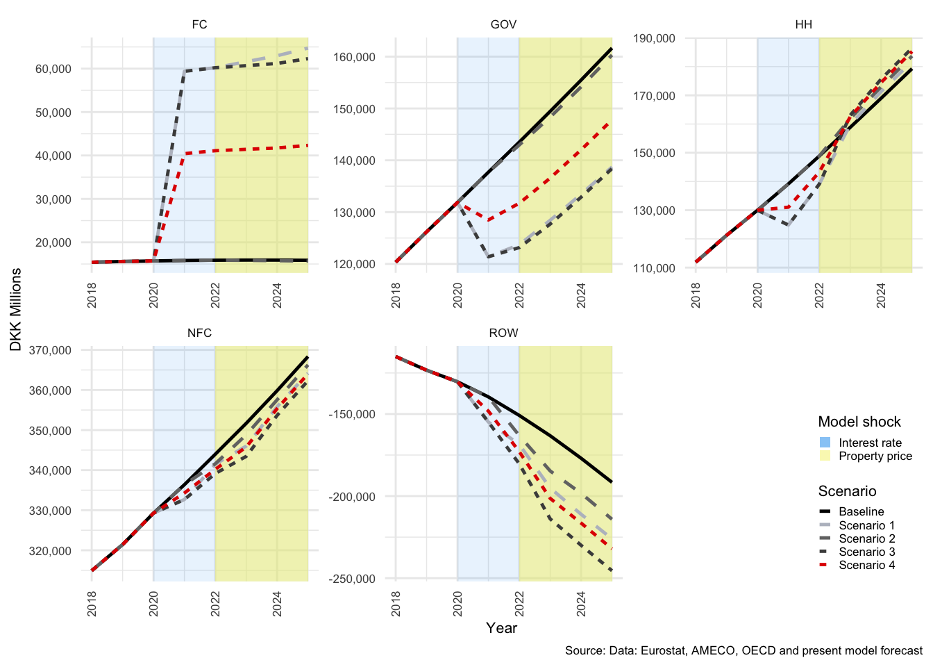
Figure 3.35: Savings

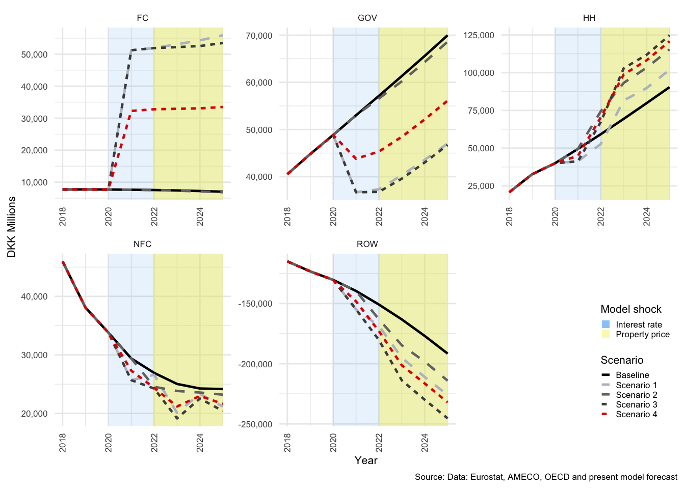
Figure 3.36: Net Lending

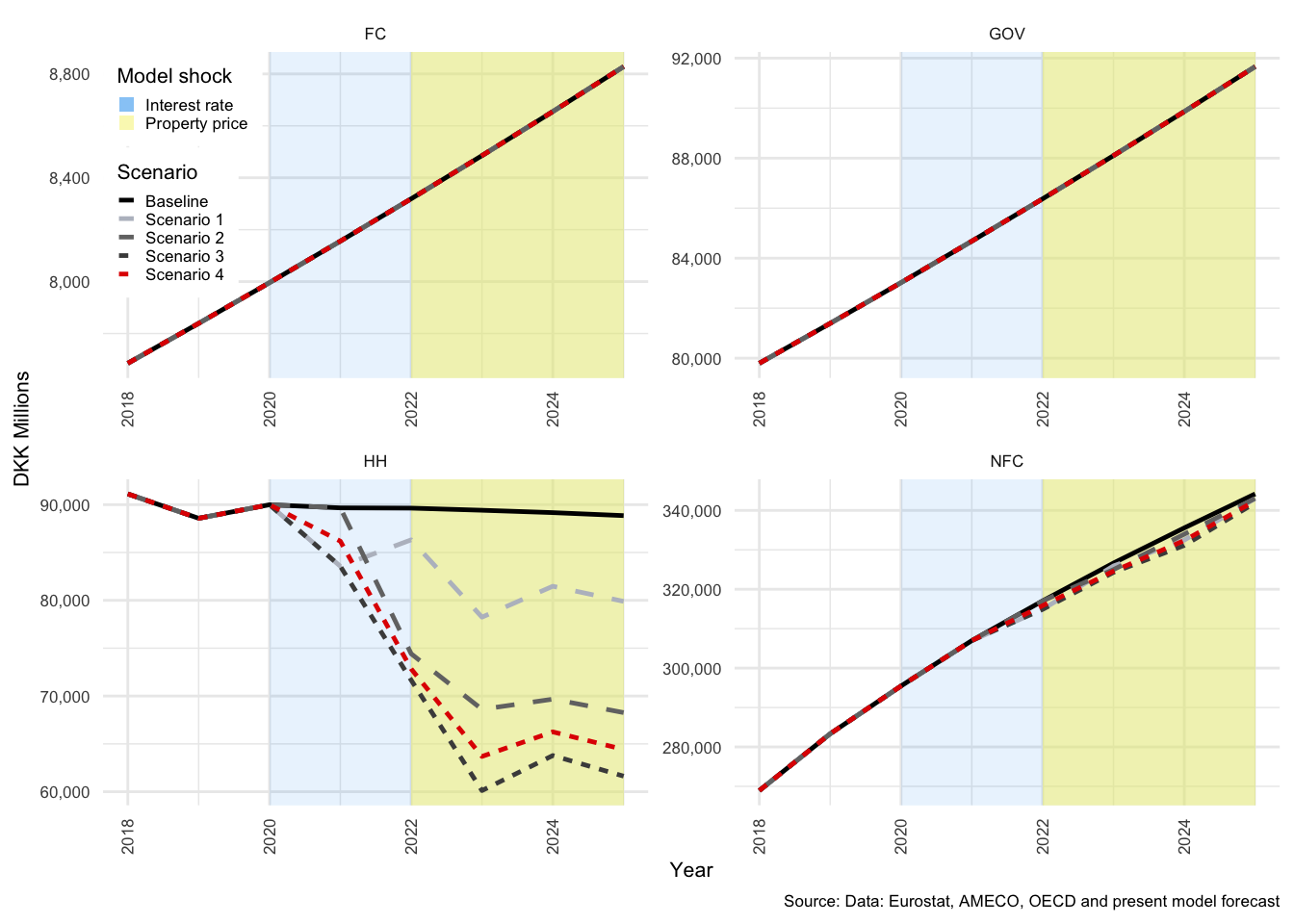
Figure 3.37: Investment

3.9.5.2 Residual sector flows

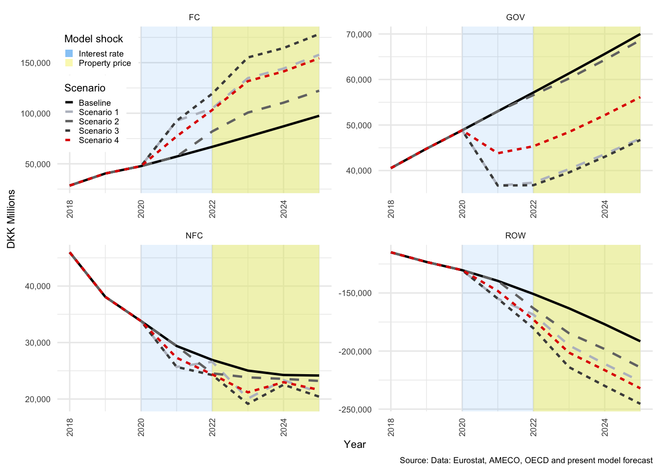
Figure 3.38: Net interest bearing asset transactions

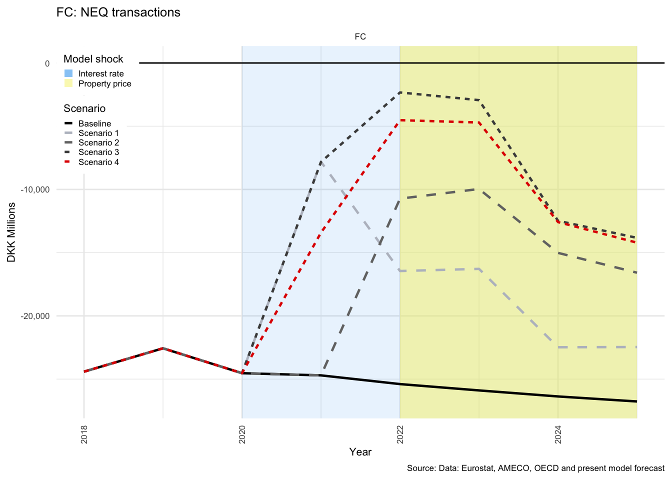
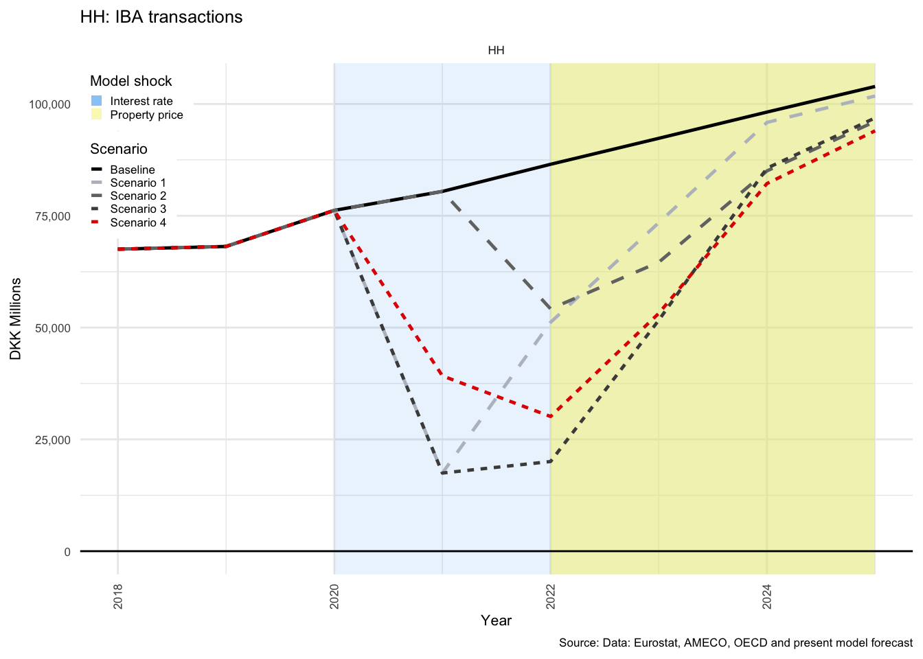
Figure 3.39: Residual flows for FC and HH

3.9.5.3 NW: Nominal prices: All sectors

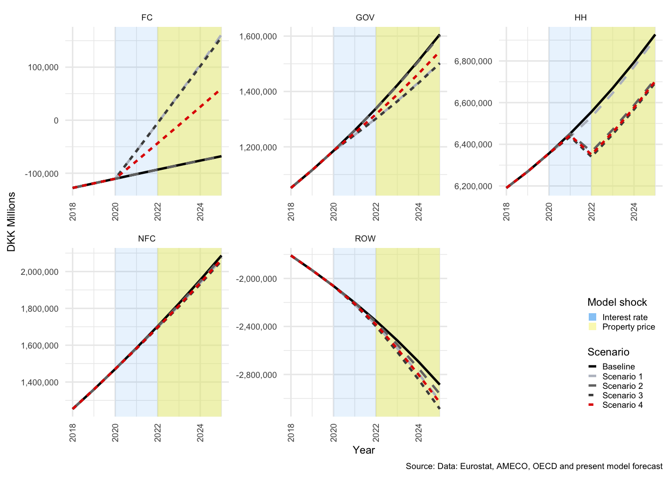
Figure 3.40: NW: Nominal prices: All sectors

3.9.5.4 Capital Stock: Nominal prices: HH, NFC

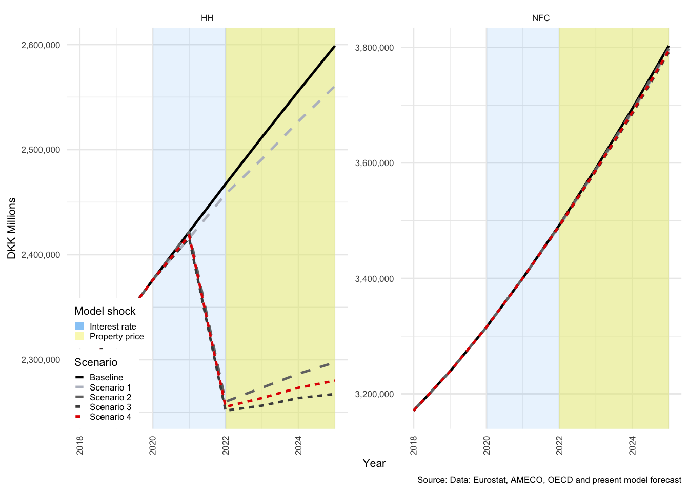
Figure 3.41: Capital Stock: Nominal prices: HH, NFC

3.9.5.5 Financial transactions: Nominal prices: HH

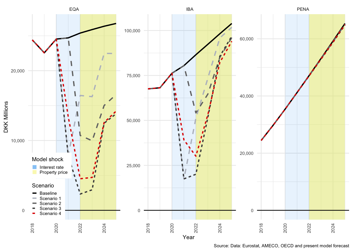
Figure 3.42: Financial transactions: Nominal prices: HH

3.9.5.6 Financial transactions: Nominal prices: NFC

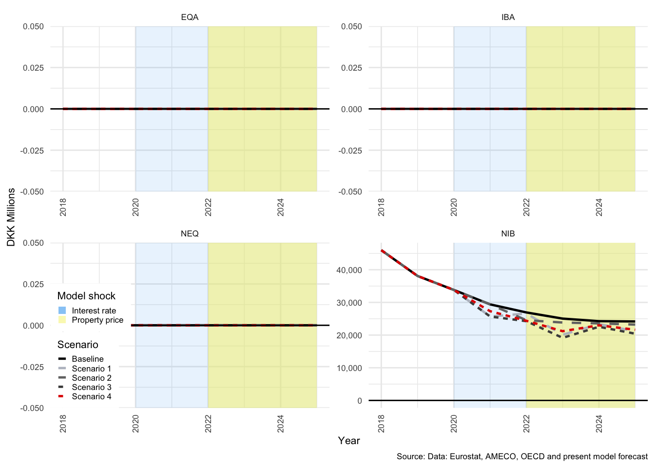
Figure 3.43: Financial transactions: Nominal prices: NFC

3.9.5.7 Financial transactions: Nominal prices: FC

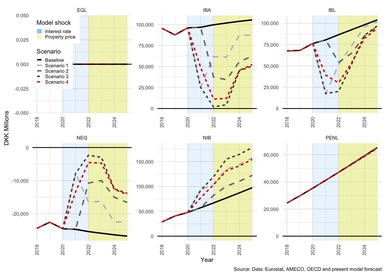
Figure 3.44: Financial transactions: Nominal prices: FC

3.9.5.8 Financial transactions: Nominal prices: GOV

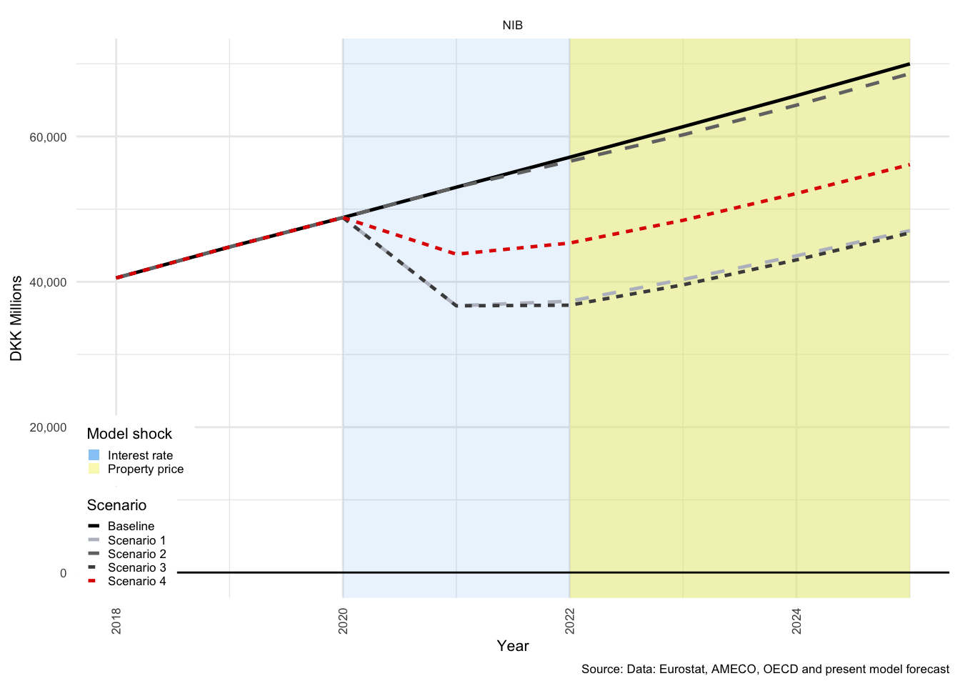
Figure 3.45: Financial transactions: Nominal prices: GOV

3.9.5.9 Financial transactions: Nominal prices: ROW

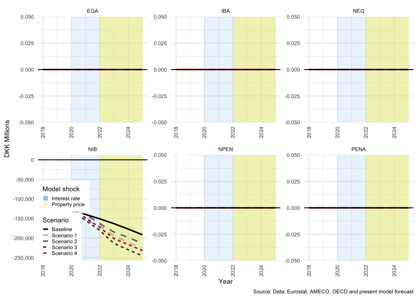
Figure 3.46: Financial transactions: Nominal prices: ROW

3.9.5.10 IBA and IBL: Stock: FC

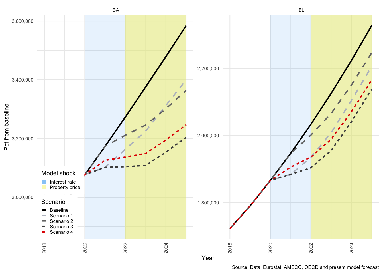
Figure 3.47: IBA and IBL: Stock: FC

3.9.5.11 IBL: Fixed and Flexible: Stocks: HH

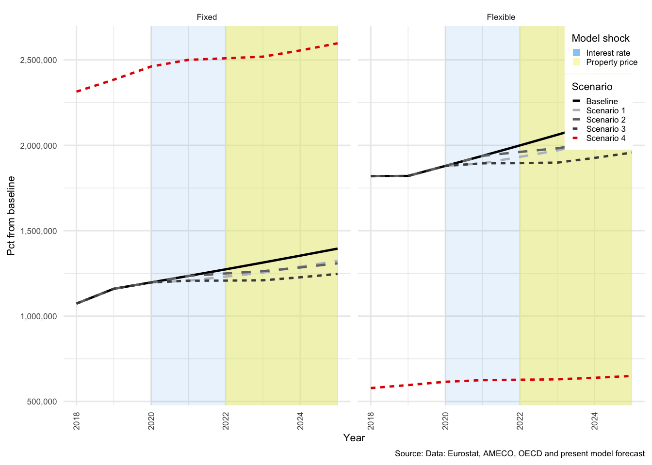
Figure 3.48: IBL: Fixed and Flexible: Stocks: HH

3.9.6 Lists of variables from scenarios

(#tab:variable-names-table_shocks)List of variables in scenario tables

Variable	Type	Description
ALPHA	Ratio	Ratio of fixed interest mortgage debt
B2	Flow	Gross operating surplus
BETA,DATA	Parameter	Parameter
BOP	Flow	Balance of payments
C	Flow	Consumption
CAB	Flow	Current account balance
CGK	Flow	Capital gains
CGS	Flow	Capital gains
CHECK,B2	Check	Consistency check: Gross operating surplus
CHECK,CTR	Check	Consistency check: Capital transactions
CHECK,EQ	Flow	Consistency check: Equity Transactions
CHECK,ERROR1	Check	Consistency check: Error 1
CHECK,ERROR2	Check	Consistency check: Error 2
CHECK,ERROR3	Check	Consistency check: Error 3
CHECK,IB	Flow	Consistency check: Interest bearing transactions
CHECK,IB,TFLOW	Check	Consistency check: Interest bearing: Flows
CHECK,INVEST	Check	Consistency check: Investment
CHECK,NEQ	Flow	Consistency check: Net equity
CHECK,NIB	Check	Consistency check: Net interest bearing
CHECK,NIB	Flow	Consistency check: Net interest bearing
CHECK,NIB,TFLOW	Check	Consistency check: Net interest bearing: Flows
CHECK,NP	Check	Consistency check: Net purchases of non-financial assets (NP)
CHECK,NPEN	Flow	Consistency check: Net pensions: Revaluations
CHECK,PEN	Flow	Consistency check: Pensions: Transactions
CHECK,STRA	Check	Consistency check: Social transfers
CHECK,TAX	Check	Consistency check: Tax
CHECK,WAGE	Check	Consistency check: Wages
CPEN	Flow	Financial Liabilities: Change in pension entitlements
CTR	Flow	Capital transfers
CU	Ratio	Capacity Utilisation (Real GNI / real capital stock)
D,1998	Dummy	Dummy variable: 1998
D,200	Dummy	Dummy variable: 2000
D,2004	Dummy	Dummy variable: 2004
D,2006	Dummy	Dummy variable: 2006
D,2007	Dummy	Dummy variable: 2007
D,2008	Dummy	Dummy variable: 2008
D,2009	Dummy	Dummy variable: 2009
D,2010	Dummy	Dummy variable: 2010
D,2011	Dummy	Dummy variable: 2011
D,2014	Dummy	Dummy variable: High taxes: 2014
D,2015	Dummy	Dummy variable: 2015
D,2016	Dummy	Dummy variable: 2016
D21	Flow	Taxes on products
D29	Flow	Other taxes on production
D31	Flow	Subsidies D31
D39	Flow	Subsidies D39
D41,P	Flow	Interest: Paid
D41,R	Flow	Interest: Received
D41B	Flow	Interest: Received
D42,P	Flow	Distributed income of corporations: Paid
D42,R	Flow	Distributed income of corporations: Received
D44,P	Flow	Other investment income: Paid
D44,R	Flow	Other investment income: Received
DELTA	Ratio	Equity to assets ratio
DEP	Flow	Depreciation of fixed capital
EQA	Flow	Financial Assets: Equity assets
EQA	Stock	Financial Assets: Equity assets
EQA,R	Ratio	Equity ratio
EQL	Flow	Financial Liabilities: Equity liabilities
EQL	Stock	Financial Liabilities: Equity liabilities
ERROR,CHECK1	Check	Error check
ERROR,CHECK2	Check	Error check
ERROR,CHECK3	Check	Error check
FA	Flow	Financial Assets
FA	Stock	Financial Assets
FAB	Flow	Financial account balance
FEE59	Ratio	Danish exports to trading partners: Weighted average total exports (imports by foreign trading partners)
FL	Flow	Financial liabilities
FL	Stock	Financial liabilities
FNL	Flow	Financial Net Lending (Balance)
FNW	Stock	Financial net wealth
G	Flow	Government expenditure
GDP	Flow	Gross domestic product
HFHF	Check	Test variable: Not used
I	Flow	Gross fixed capital formation
IBA	Flow	Financial Assets: Interest bearing assets
IBA	Stock	Financial Assets: Interest bearing assets
IBL	Flow	Financial Liabilities: Interest bearing liabilities
IBL	Stock	Financial Liabilities: Interest bearing liabilities
IBL,RV1	Flow	Financial Liabilities: Interest bearing liabilities
INFL	Rate	Inflation rate: Price inflation
INFL,M	Rate	Inflation rate: Price inflation: Foreign
INV	Flow	Gross fixed capital formation
K	Stock	Stock of Capital
K,CG	Flow	Capital Gains
KCG	Flow	Capital Gains
KCG,SUM	Flow	Capital Gains - Cummulative sum
LEV	Ratio	Leverage ratio: NFC: Funding liabilities to GDP
LEV1	Ratio	Leverage ratio: NFC: Funding liabilities
LF	Stock	Labour force: Total number of employable persons
M	Flow	Imports
N	Stock	Labour force: Denmark for workers in production
NEQ	Flow	Net financial stock: Equity
NEQ	Stock	Net financial stock: Equity
NF	Stock	Labour force: Employed persons: Danish waged
NIB	Flow	Net financial stock: Interest bearing
NIB	Stock	Net financial stock: Interest bearing
NL	Flow	Sector Balance
NL,CHECK	Check	Consistency check: Net lending
NP	Flow	Net purchases of non-financial assets (NP)
NPEN	Flow	Net financial stock: Pension
NPEN	Stock	Net financial stock: Pension
NPIR	Flow	Net property income received: Total
NPIR,NEQ	Flow	Net property income received: NEQ
NPIR,NIB	Flow	Net property income received: NIB
NPIR,NPEN	Flow	Net property income received: NPEN
NU	Stock	Labour force: Employed persons: Danish nationals: Employed abroad
NW	Stock	Net Wealth
NX	Flow	Net Exports
OTR	Flow	Other current transfers
P,CGK	Deflation index	Price index: Capital gains
P,NEQ	Deflation index	Price index: Net Equity
P,NIB	Deflation index	Price index: Net interest bearing assets
P,PEN	Deflation index	Price index: Pensions
PC	Deflation index	Price deflator: Consumption
PE	Deflation index	Price deflator: Unknown
PENA	Flow	Financial Assets: Pension assets
PENA	Stock	Financial Assets: Pension assets
PENL	Flow	Financial Liabilities: Pension liabilities
PENL	Stock	Financial Liabilities: Pension liabilities
PG	Deflation index	Price deflator: Government consumption
PH	Deflation index	Price deflator: Houses
PH01	Deflation index	Price deflator: Houses (Alternative)
PHI1	Flow	Social contributions to income
PHI2	Flow	Pension transactions to social contributions
PI	Deflation index	Price deflator: Investment (weighted average of deflators for housing(pk) and all other investment (pk)) . Proportion of dwellings in total investment is approx 0.22, and pi closely resembles the deflator for total investment reported by ameco.
PIP	Flow	Property income paid
PIP,IBL	Flow	Property income paid: IBL
PIP,PENL	Flow	Property income paid: PENL
PIR	Flow	Property income received
PIR,EQA	Flow	Property income received: EQA
PIR,IBA	Flow	Property income received: IBA
PIR,PENA	Flow	Property income received: PENA
PK	Deflation index	Price deflator: Investment (excluding dwellings)
PM	Deflation index	Price deflator: Imports
PNFC	Deflation index	Price deflator: NFC K
POP	Stock	Population
PP	Check	Unknown
PRIVATE	Flow	Gross income
PROD	Stock	Labour Force: Labour productivity
PROFIT	Ratio	Profit share (Residual of wage share)
PX	Deflation index	Price deflator: Exports
PY	Deflation index	Price deflator: GDP
R,EQ	Rate	Rate of return: Equities
R,ERROR1	Check	Property income error
R,ERROR2	Check	Property income error
R,ERROR3	Check	Property income error
R,IBA	Rate	Rate of interest: Interest bearing assets
R,IBL	Rate	Rate of interest: Interest bearing liabilities
R,IBL,SENS	Rate	Rate of interest: Interest bearing liabilities: Weighted mortgage interest rate
R,N	Rate	Rate of return: Mean
R,NET,ERROR1	Check	Property income error
R,NET,ERROR101	Check	Property income error
R,NET,ERROR2	Check	Property income error
R,NET,ERROR201	Check	Property income error
R,NET,ERROR3	Check	Property income error
R,NET,ERROR301	Check	Property income error
R,PEN	Rate	Rate of return: Pensions
R,R,IBL	Rate	Rate of interest: Interest bearing liabilities
RHO	Ratio	Equity ratio
RR	Rate	Rate of return
S	Flow	Savings
SBE	Flow	Social benefit transfers
SCO	Flow	Social benefit contributions
STRA	Flow	Social transfers
T	Flow	Taxes on products
TAX	Flow	Tax
TEST	Check	Test variable: Stock of Capital (Change in)
TOBIN,Q	Index	Index: House price index: Tobin’s Q = Ratio between the house price index and the construction cost of housing index
TOP	Ratio	Ratio of foreign to domestic trade
UL,COST	Rate	Labour force: Unit labour cost
ULC	Rate	Labour force: Unit labour cost: Price index: Index for the price deflator with reference to 2010 (all other price deflator indices are referenced to 2010)
UN	Stock	Labour force: Unemployed persons
UR	Ratio	Labour force: Unemployment rate
W	Flow	Wages
WAGE	Rate	Labour force: Wage rate
WI	Rate	Inflation rate: Wage inflation
WS	Ratio	Wage share
X	Flow	Exports
XR	Rate	Exchange rate
Y	Flow	Total income
Y,D	Flow	Disposable Income
YEAR
ZZ	Index	Index: House price index
ZZ,I	Index	Index: House price: Imported from DST
ZZ,INDEX	Index	Index: House price: Mark-up pricing on construction costs
ZZ1	Index	Index: House price: Imported from DST

3.10 Complete set of model equations

3.10.1 Non-Financial Corporate Sector

The following appendix is adapted from Byrialsen and Raza (2019), except otherwise indicated. It is included here for completeness in the explanation of the structure of the model. As in their model, the non-financial corporate sector (NFC) is responsible for all production, where total nominal production is represented as:

\[\begin{equation} Y_t = C_t + I_t + G_t + X_t - M_t \label{eq:ynominal} \end{equation}\]

This can be rewritten in terms of sales, or rather, from an income perspective:

\[\begin{equation} S_t = C_t + I_t + G_t + X_t \label{eq:nfcsales} \end{equation}\]

The production equation from Equation () can be deflated to real prices;

\[\begin{equation} y_t = c_t + i_t + g_t + x_t - m_t \end{equation}\]

Where the GDP deflator can be represented as:

\[\begin{equation} P^y_t = \frac{Y_t}{y_t} \end{equation}\]

Outflows for NFC include taxes paid to GOV, wages (\(WB\)) paid to domestic and foreign households, and profits (\(B2\)⁴²).

\[\begin{equation} WB^N_t = W_t(N^N_t) \end{equation}\]

The nominal wage bill is calculated as the wage rate (\(W_t\)) times the level of employment (\(NN_t\)), where \(NN_t\) includes all domestic employment of citizens plus the net employment of foreigners in Denmark and Danish citizens abroad.

Taxes paid by NFC are predominantly production based and are therefore calculated as a proportion of total production in each period (\(Y_t\)).

\[\begin{equation} T^N_t = \beta _3(Y_t) \end{equation}\]

It is assumed that firms target a fairly stable level of mark-up on production, and thus \(B2\) is calculated as an estimated proportion of \(Y_t\).

\[\begin{equation} B2_t = \beta Y_t \end{equation}\]

The stock of NFC fixed capital, (\(K^N_t\)), is diverse, and is calculated via the standard accounting method, allowing for capital accumulation via investment (\(I^N_t\)), depreciation (\(D^N_t\)) and capital gains (\(K^N_{CG_t}\)).

\[\begin{equation} K^N_t = K^N_{t-1} + I^N_t - D^N_t + K^N_{CG_t} \end{equation}\]

Depreciation of capital is assumed to apply to stock held at the end of the previous period.

\[\begin{equation} D^N_t = \delta (K^N_{t-1}) \end{equation}\]

The capital deflator (\(P^i_t\)) can then be used to calculate the real value of the stock of capital in each period.

\[\begin{equation} k^N_t = \frac{K^N_t}{P^i_t} \label{eq:realcap} \end{equation}\]

Investment is estimated in real terms as a function of capacity utilisation.

\[\begin{equation} ln(i^N_t) = \beta _i + ln\beta _i. \Bigg( \frac{y_{t-i}}{k^N_{t-i}}\Bigg) \end{equation}\]

It can then be inflated to current prices using the same capital price deflator as in Equation (), \(P^i_t\).

\[\begin{equation} I^N_t = i^N_t(P^i_t) \end{equation}\]

NFC savings (\(S^N_t\)), not to be confused with sales (\(S_t\)) in Equation (), can be calculated as the net sum primary and secondary income and expenditures.

\[\begin{equation} \begin{split} S^N_t = & Y_t - WB^N_t + (B2^N_{t} - B2_{t}) + r^N_{t-1}(NIB^N_{t-1})\\ & + \chi _t (NEQ^N_{t-1}) - T^N_t + STR^N_t + \epsilon ^N \end{split} \end{equation}\]

Net lending (\(NL^N\)) takes into account the additional sources of change originating from fixed asset adjustments. In particular, \(NP\) is the net sale and acquisition of non-financial assets, savings and investment reflect ex post portfolio decisions, and finally \(KTR^N\) represents any additional capital transfers.⁴³ NFC is also assumed to receive all income from production in the economy, and thus the level of operating surplus must be adjusted to take into account that of all other sectors, thus NFC retains (\(B2^N_{t} - B2_{t}\)) gross operating surplus. The \(\epsilon ^N\) refers to adjustments made to ensure stock and flow consistency in the level of property income received or paid during the periods where data was available⁴⁴.

\[\begin{equation} NL^N_t = S^N_t - I^N_t- NP^N_t + KTR^N \end{equation}\]

The calculation of stocks for each of the classes held by NFC are in equations () and ().

Net equities:

\[\begin{equation} NEQ^N_t = NEQ^N_{t-1} + NEQTR^N_t + NEQ^N_{CG_t} \label{eq:nfc-neq} \end{equation}\]

Net interest bearing stocks:

\[\begin{equation} NIB^N_t = NIB^N_{t-1} + NIBTR^N_t + NIB^N_{CG_t} \label{eq:nfc-nib} \end{equation}\]

Net interest bearing assets, like several others in this model, are determined by a combination of previous stocks (\(NIB^N_{t-1}\)), transactions (\(NIBTR^N_t\)) and capital gains (\(NIB^N_{CG_t}\)). The transactions component of interest bearing assets for NFC is determined passively. It is calculated as the remainder of Savings, after capital transfers, and after portfolio allocation towards equities. Transactions in equities (\(NEQTR^N\)) are thus the active component of the composition of the NFC balance sheet portfolio.

\[\begin{equation} NIBTR^N_t = NL^N_t - NEQTR^N_t \end{equation}\]

Since NFC only holds these two financial assets in the model, the sum constitutes the financial net wealth (\(FNW^N\)) of NFC.

\[\begin{equation} FNW^N_t = NIB^N_t + NEQ^N_t \end{equation}\]

This is different to the total net wealth (\(NW^N\)), which also includes the fixed capital (\(K^N\)) owned by NFC.

\[\begin{equation} NW^N_t = FNW^N_t + K^N \end{equation}\]

3.10.2 Household Sector

The household sector (HH) is the primary focus of this model, in particular the interest bearing liabilities of the household sector, and the drivers thereof. It is therefore the sector with most endogenous components. Equation () describes the incomes and expenditures of HH. The primary sources of which are wages (\(WB^H\)), profits (\(B2\)), property income (or returns on financial capital, which stems from interest bearing assets, \(IBA^H\), pensions, \(PENA^H\), and equities, \(EQA^H\)), and social transfers(\(STR^H\)).

\[\begin{equation} \begin{split} Y^H_t = & WB^H_t + B2^H_{t} + r^H_{A_{t-1}}(IBA^H_{t-1})\\ & - r^H_{L(FI)_{t-1}}(IBL(FI)^H_{t-1})\\ & - r^H_{L(FL)_{t-1}}(IBL(FL)^H_{t-1})\\ & + \chi _t(EQA^H_{t-1}) + \psi _t(PENA^H_{t-1}) + STR^H_t + \epsilon ^H \label{eq:Yht} \end{split} \end{equation}\]

Interest rates are represented by \(r^H\), and the “A” (“L”) subscript referring to the assets (liabilities), and (\(\chi _t\)) and (\(\psi _t\)) are the rates of return on equities and pensions. As part of the key change in this model, the level of interest paid on \(IBL\) in this model is split between fixed and flexible rate mortgages into \(r^H_{L(FI)_{t-1}}(IBL(FI)^H_{t-1})\) and \(r^H_{L(FL)_{t-1}}(IBL(FL)^H_{t-1})\). A similar split is present in the financial corporate sector (FC) below.

Social transfers received by the households in the above equations is the sum of social contribution (\(SCON^H\)) paid by the households, social benefits (\(SBEN^H_t\)), and other transfers (\(OTR^H\)) received by the households: Social transfers:

\[\begin{equation} STR^H_t = SBEN^H_t + OTR^H_t - SCON^H \end{equation}\]

Total taxes paid by households are a relatively constant proportion of income over time, and are deducted from total income to give disposable income:

\[\begin{equation} YD^H_t = Y^H_t - T^H_t \end{equation}\]

The total value of tax payment by households is assumed to be a constant portion (\(\beta _i\)) of household primary and secondary income.

\[\begin{equation} T^H_t = \beta _i (Y^H_t) \end{equation}\]

The level of social contributions are a proportion of disposable income, adjusted over time.

\[\begin{equation} SCON^H_t = \beta _7(YD^H_{t-i}) \end{equation}\]

The largest components of \(SBEN^H\) are pension and medical payments. Byrialsen and Raza (2019), modelled changes in benefits against changes in the the wage rate and the level of unemployment. Although not directly related to the main components of benefits, they appear to be good proxies for changes in pension distributions, which in some cases may be based on emoluments.

\[\begin{equation} ln(SBEN^H_t) = \beta _i + \beta _i ln(U^N_t) + \beta _i ln(W^H_{t-i}) \label{eq:socialbenefits} \end{equation}\]

Since 2007, approximately 35% - 37% of all social benefits were for old age payments. A further 20% - 22.3% are attributed to medical benefits, an almost constant 14.4% to disability and 10% - 13.2% to family and child benefits. Unemployment (app. 5%), social exclusion (app. 5%), housing (app. 2%) and survivorship (app. 1%) benefits making up the balance.

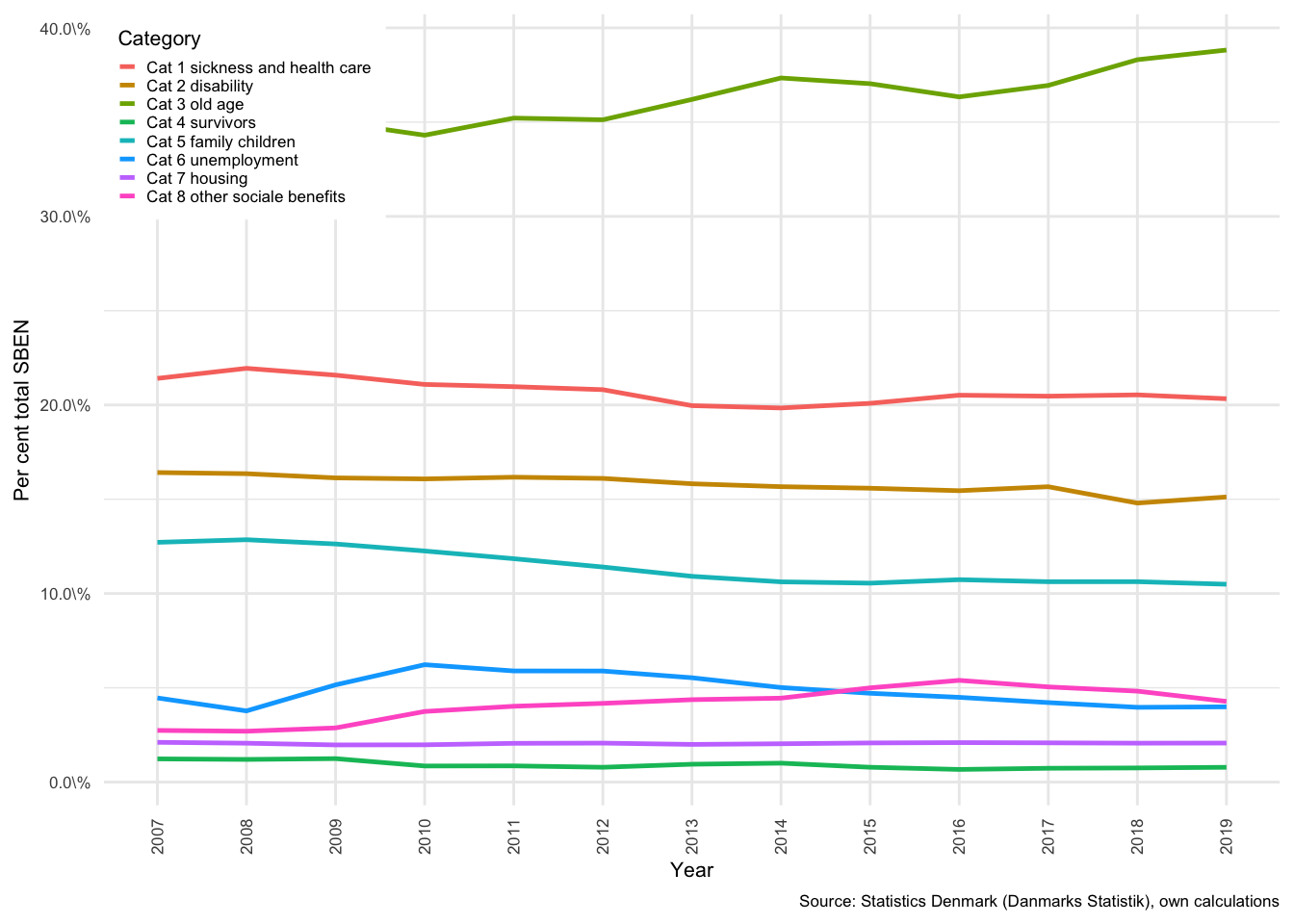
Figure 3.49: Social benefits by category

The old age category, as can be seen from Figure , is then dominated by tax funded pension payouts (app. 50% in 2017), old age accommodation and care (app. 15%) and civil (app. 11%) and other pension schemes (app. 12%), with the declining anticipated pension allocations (app. 5.2% in 2017) and growing labour market supplementary pension benefits (ATP⁴⁵) (app. 5.8%) making up the balance. The full amount therefore could be considered as pension income, but since these pension benefits are funded predominantly by tax, rather than from assets, they are best kept separate from the capital income on pension assets described in Equation () above. This is perhaps with the exception of labour market supplementary pension benefits, which are payouts from a pooled investment portfolio.

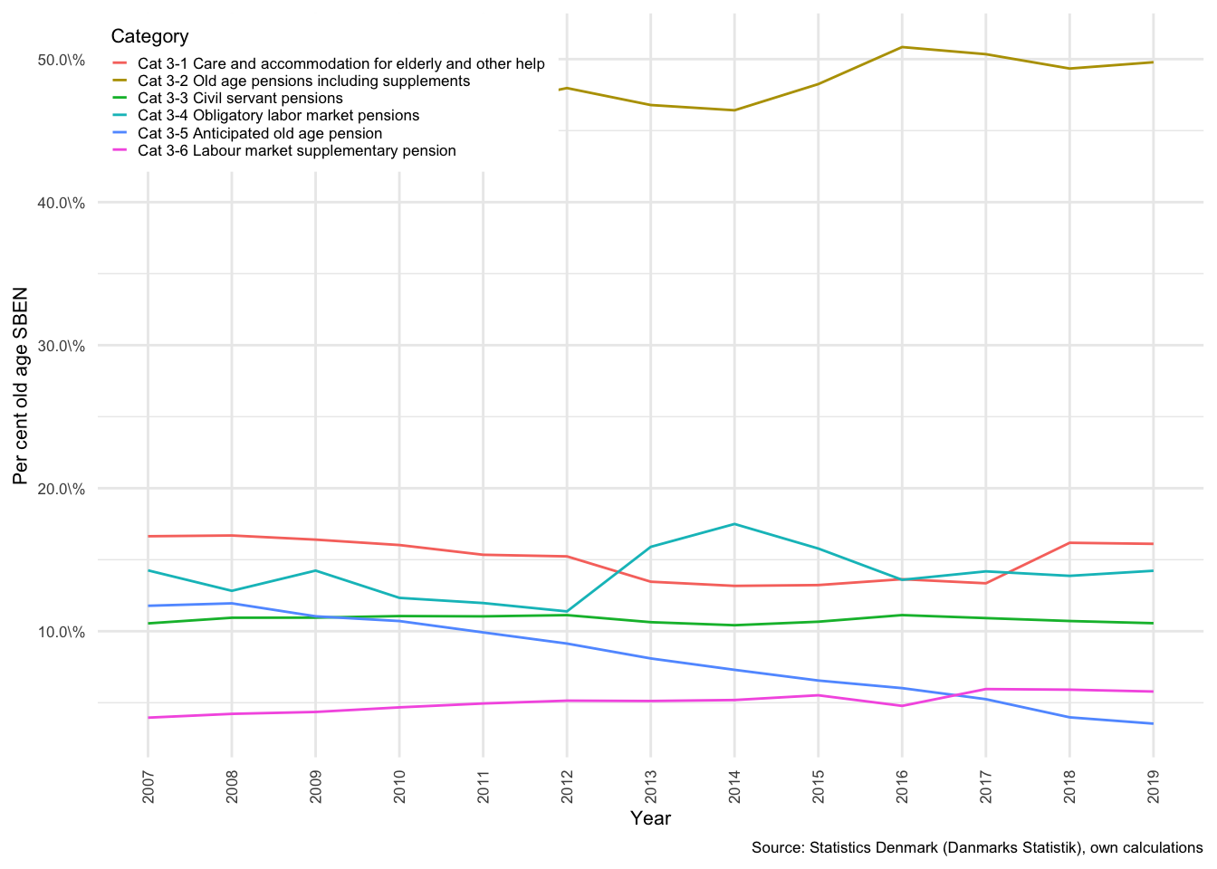
Figure 3.50: Old age social benefits

This is not merely a question of semantics, as the old age component is also an element of wage negotiations for the working population. A large part of social contributions (\(SCON^H\)) are also contributions towards the labour market pension fund.⁴⁶ \(SBEN^H\) is, perhaps understandably, the second largest component of HH disposable income in Denmark. As can be seen in Figure , this can quickly be understood to be driven primarily by healthcare and pensions, but in a more general sense, by components of the strong Danish welfare system. Labour market pension payouts are expected to fall (rise), as are unemployment benefit payouts, as economic conditions improve (deteriorate). Unemployment, as an indicator of economic distress, appears to be a good proxy for expected changes in benefit payouts relative to total HH disposable income. Equation () captures this effect, together with the effect of changes in the wage rate. The latter because unemployment benefits and several pension benefits are adjusted according to changes in industry wage rates, as noted by Byrialsen and Raza (2018) and (2019).

Real disposable income, as will be the case for several other variables in this model, can be calculated by dividing household disposable income by a consumption price index (\(P^c\)).

\[\begin{equation} yd^H_t = \frac{YD^H_t}{P^c_t} \end{equation}\]

Consumption, like NFC investment, is estimated in real terms in a standard Keynesian form, and log-linearised for stationarity. Consumption is taken to be determined by a combination of real disposable income and household wealth of the preceding period. Although not explicitly modelled, current consumption thus is assumed to be based purely on expectations developed in the previous period.

\[\begin{equation} ln(c_t) = \beta _0 + \beta _iln(yd^H_{t-i}) + \beta _iln(nw^H_{t-1}) \label{eq:hh_consumption} \end{equation}\]

Nominal consumption can be calculated using the consumption price index to inflate the series.

\[\begin{equation} C_t = c_t(P^c_t) \end{equation}\]

\(P^c\), the consumption price index is endogenous to changes in the wage rate and the import price index from the previous period. In some way reflecting a delayed adjustment in (or, sticky) prices, and the importance of international prices for smaller open economies, such as Denmark.

\[\begin{equation} ln(P^c_t) = \beta _0 + \beta _iln(W_{t-i}) + \beta _iln(P^m_{t-i}) \end{equation}\]

The following equations are related to household interactions with capital an investment markets.

In this model, households are only permitted to make productive investment in housing, which, in this model, is considered only as a primary market, following G. Zezza (2008), Fontana and Godin (2013) and Beckta (2015). The secondary market for houses is assumed to affect prices, but not the demand for additional housing investment. Demand for housing investment is determined by by a Tobin’s-Q-like function, partially driven by changes in disposable income and previous period housing investment, and partially driven by a relative shift in sales price (\({P^H_{t-i}}\)) and construction cost (\({P^i_{t-i}}\)) indices.

Real investment in fixed assets (dwellings):

\[\begin{equation} ln(i^H_t) = \beta _i + \beta _i ln(i^H_{t-i}) + \beta _i ln \Bigg( \frac{P^H_{t-i}}{P^i_{t-i}}\Bigg) + \beta _iln(yd^H_{t-i}) \label{eq:housing-hh} \end{equation}\]

As noted by Byrialsen and Raza (2019, 20), “The intuition behind the above equation is straight forward, i.e., an increase in the house prices motivates the households to invest more in the construction of new houses, while an increase in the construction costs would lower housing investment.”

A shift downwards in house prices would conversely reduce overall returns on houses relative to construction costs, and thus result in a decline in the demand for housing investment. This would result, all else equal, in an increase in savings and a consequent rise in the demand for alternative outlets. Limited below to the purchase of financial assets⁴⁷.

The nominal level can be calculated by inflating the real investment in housing series (\(i^H_t\)) by the investment price index (\(P^i_t\)):

\[\begin{equation} I^H_t = i^H_t(P^i_t) \end{equation}\]

The nominal stock of housing (\(K^H\)), as with other assets to come, follows the simple process of previous stock, plus acquisition (in this case investment in new houses), less depreciation (or disposal) plus capital gains.

\[\begin{equation} K^H_t = K^H_{t-1} + I^H_t - D^H_t + K^H_{CG_t} \end{equation}\]

Capital gains on houses, in turn, are calculated as:

\[\begin{equation} KH_{CG} = \Delta P^H_t (K^H_{t-1}) \end{equation}\]

Which is simply the change in the price of houses applied to the level of stock at the end of the preceding period. The change in house prices leading into the current period is then by definition the same ratio proportion of capital gains to previous housing capital.

\[\begin{equation} \Delta P^H_t = \frac{KH_{CG}}{K^H_{t-1}} \label{eq:changehouseprice} \end{equation}\]

Nominal housing capital held by HH at the end of the current period can be expressed as the price adjusted stock at the end of the previous period, plus net investment and depreciation.

\[\begin{equation} K^H_t = K^H_{t-1}(1 + \Delta P^H_t) + I^H_t- D^H_t \end{equation}\]

The deflated real capital index can then be found by dividing the series by the investment (housing) price index, as in Equation () above.

\[\begin{equation} k^H_t = \frac{K^H_t}{P^i_t} \end{equation}\]

The level of savings is then calculated as a residual disposable income after consumption and net pension adjustments - the ESA 2010 (Statistical Office of the European Communities. 2013) definition of which is net of contributions, disbursements and returns of pension funds.

\[\begin{equation} S^H_t = YD^H_t - C^H_t + CPEN^H_t \end{equation}\]

Net lending can then be calculated savings plus additional consideration for the net acquisition and disposal of fixed assets (\(NP\)) and capital transfers (\(KTR\)) less investment (assumed here to be solely in houses).

\[\begin{equation} NL^H_t = S^H_t - I^H_t - NP^H_t + KTR^H_t \end{equation}\]

HH must also fund real activities and allocate any excess funds in the financial markets. As noted above, HH is the sector with most endogenous components in this model. It is also the sector, together with the financial corporate sector (FC) that has the most complex financial accounts. As noted by Byrialsen and Raza (2019), financial market changes in this model are driven primarily by the demand for credit and assets. As they explained, transmission is from flows to stocks. The behaviour is primarily modelled in transaction decisions, and stocks are then calculated as the sum of these together with capital gains.

The net effect of annual changes in the financial position of HH is captured by financial net lending. This is the sum of changes in financial assets less the sum of changes in financial liabilities:

\[\begin{equation} FNL^H_t = FATR^H_t - FLTR^H_t \end{equation}\]

Household financial assets are held in interest bearing assets (\(IBA\)), equities⁴⁸ (\(EQA\)) and pensions (\(PENA\)). Transactions in each of these sum to make up the total transactions in financial assets.

\[\begin{equation} FATR^H_t = IBATR^H_t + EQATR^H_t + PENATR^H_t \end{equation}\]

Transactions in equities are determined by a Tobin allocation matrix, thus enforcing a budget constraint on HH, where the investment decision of the sector is determined at least in part by relative rates of return. One exception is pension allocations, where a fairly constant portion of HH income is allocated to pension investments, irrespective of the rate of return. This leaves equities and interest bearing assets.

Demand for equities is negatively affected by increases in the returns available on interest bearing assets in the previous period (\(\beta\) on \(r^H_{A_{t-1}}\)), positively related to returns on equities (\(\chi\)), and positively related to increases in the extension of credit (\(\beta\) on \(IBLTR^H\)).

\[\begin{equation} EQATR^H_t = \beta _i + \beta _i(\chi _t) + \beta _i(r^H_{A_{t-1}}) + \beta _i(IBLTR^H_t ) \end{equation}\]

The link with \(IBL\) is associated with the investment incentive for more sophisticated investors, where low interest rate debt can be used to arbitrage higher returns on equities.

Pension transactions, in addition to the fixed proportion that is reflected as a constant in the equation below, are positively affected by returns on pensions (\(\psi\)) and the wage bill (\(WB\)). Pensions transactions can thus be affected directly by the wage rate, or the level of employment (and thus negatively by a rise in unemployment).

\[\begin{equation} PENATR^H_t = \beta _i + \beta _i(\psi _t) + \beta _iWB^H_t \end{equation}\]

The demand for credit by households is where the current model differs most from Byrialsen and Raza (2019). The total demand for new credit is captured in the level of transactions (\(IBLTR^H\)). This is positively related to the level of demand for (new) housing (\(I^H\)), negatively to the level of debt in the previous period, positively to the total level of transactions in equities (for the same investment reason described above), and negatively related to the interest cost on loans (\(r^H_{L_{t-1}}\)) in the previous period.

\[\begin{equation} IBLTR^H_t = \beta _i(I^H_{t-i}) + \beta _i(IBL^H_{t-i}) + \beta _i(FATR^H_t) + \beta _i(r^H_{L_{t-1}}) \end{equation}\]

The primary change to the model is the introduction of adjustable rate mortgage products in a fairly generic form, where the total level of outstanding \(IBL\) is split into fixed-interest (\(IBL_{FI}\)) and flexible-interest bearing liabilities (\(IBL_{FL}\)). The proportion of interest bearing assets held as \(IBL_{FI}\) is \(\alpha\).

\[\begin{equation} IBL^H_{FI_t} = \alpha(IBL^H_t) \end{equation}\]

and thus,

\[\begin{equation} IBL^H_{FL_t} = (1-\alpha)(IBL^H_t) \end{equation}\]

The level of \(\alpha\) is taken from Statistics Denmark, and varies over time. The split is introduced in 2003, when the option was made available to HH. The composition of this debt is significantly more complex, as discussed in Section above. This complexity can be simplified using a combination of interest rates and sensitivity or adjustment weights. At an aggregate level, the degree to which flexible rate mortgages adjust to changes in official rates can be estimated for each aggregate group of mortgage products. This is done for two broad groups in for this model, fixed⁴⁹ and flexible⁵⁰. The effect is calculated as a percentage pass-through of official rate changes. Unfortunately it is not possible to compare rising and falling pass-through rates to existing mortgage holders prior to 2009. For the 2009 to 2017 period, however, fixed and flexible average interest rate payments, relative to outstanding nominal capital (cash) amounts, appears to have followed a very stable spread of approximately 2%. This is fairly easy to explain in a falling rates environment as borrowers take advantage of the option to refinance debt.

The composition of debt and the expected pass-through rate have a combined effect on the sensitivity of HH balance sheets and incomes to a shock to either interest rates or property prices. This simple modification is able to capture the two most dramatics innovations in the Danish mortgage debt system: the introduction of ARMs and of delayed amortization (or interest-only period, IO loans) loans.

The incentive to borrow for the purchase of a house, as in Equation () above, is partially driven by interest rates. The available interest rate is then adjusted according to the weighted average interest rate observed for each of the two groups (flexible and fixed). The second is the introduction of interest-only periods, as explained in Section , the effect of which is to reduce the initial cost of borrowing. Thus as the amount paid on mortgages per family falls, the incentive to borrow rises.

An alternative is to calculate the interest rate as the total payments made by the household towards debt, inclusive of amortization payments, as a percentage of total debt remaining. This alternative is not employed here, but is planned for future research. Although this would not normally be captured in the interest rate, it is possible to artificially lower the rate of interest on the flexible rate group in order to capture this incentive. This is similar for debt with longer term structures, where monthly costs would reflect the reduced portion allocated to amortization.

Unfortunately, the additional risks factors related to products with full-term interest-only, or perpetual-interest-only loans would not be possible to capture in this framework.

The only interest bearing asset held by households in the model is deposits, which are calculated as the residual effect of transactions in the other assets. debt and net lending contributing positively, and outflows for equities or pension investment contributing negatively.

\[\begin{equation} IBATR^H_t = NL^H + IBLTR^H_t - EQATR^H_t - PENATR^H_t \label{eq:ibatr_hh} \end{equation}\]

The current stock of each asset is then the sum of the stock from the preceding period, plus any transactions (positive or negative), plus any capital gains (or losses). The same is true for all assets and liabilities.

\[\begin{equation} IBA^H_t = IBA^H_{t-1} + IBATR^H_t + IBA^H_{CG_t} \end{equation}\]

Equities:

\[\begin{equation} EQA^H_t = EQA^H_{t-1} + EQATR^H_t + EQA^H_{CG_t} \end{equation}\]

Pensions:

\[\begin{equation} PENA^H_t = PENA^H_{t-1} + PENATR^H_t + PENA^H_{CG_t} \end{equation}\]

Interest bearing liabilities:

\[\begin{equation} IBL^H_t = IBL^H_{t-1} + IBLTR^H_t + IBL^H_{CG_t} \end{equation}\]

The sum of financial assess (liabilities) provides the total financial assets (liabilities).

\[\begin{equation} FA^H_t = IBA^H_t + EQA^H_t + PENA^H_t \end{equation}\]

Since the only financial liability for households in this model interest bearing, it makes up the total.

\[\begin{equation} FL^H = IBL^H_t \end{equation}\]

Net financial wealth is the difference between total assets and liabilities.

\[\begin{equation} FNW^H_t = FA^H_t - FL^H_t \end{equation}\]

The inclusion of fixed assets provides the total net wealth for each sector, which both in this model and in reality are dominated by dwellings for the household sector.

\[\begin{equation} NW^H_t = FNW^H_t + K^H_t \end{equation}\]

This can be deflated to provide wealth at constant prices, where real financial net wealth:

\[\begin{equation} fnw^H_t = \frac{FNW^H_t}{P^c_t} \end{equation}\]

And, where real wealth, are the result of deflation by the consumption prices index \(P^c_t\)

\[\begin{equation} nw^H_t = \frac{NW^H_t}{P^c_t} \end{equation}\]

3.10.3 Financial Corporate Sector

The financial sector acts as the provider, and thus counterpart of newly created credit in this model. The financial corporate sector (FC) is comprised of banks, insurance and pension companies, as well as several services related to the financial markets. Property income made up just below 75% of FC inflows, and approximately the same proportion of outflows in 1995, and falling to just above 50% in 2017 - with positive flows higher than negative flows, reflecting the rental income spread extracted by the sector.

Savings, according to the national accounts can be expressed as the sum of the net capital income, gross operating surplus (\(B2^F_t\)) (received), social transfers (\(STR^F\)) minus taxes paid to the government (\(T^F\)), and the changes in pension entitlements (\(CPEN^F\)) paid to the households.

This model adjusts the inflow to FC to take into account the split in debt in the household sector between flexible and fixed, where the average interest rate on each category is applied to the outstanding level of fixed or flexible debt respectively.

\[\begin{equation} \begin{split} S^F_t = & B2^F_t \\ & + r^F_{A(FI)_{t-1}}(IBA^{F\sim H}_{A(FI)_{t-1}}) + r^F_{A(FL)_{t-1}}(IBA^{F\sim H}_{A(FL)_{t-1}}) \\ & - r^F_{L_{t-1}}(IBL^{F\sim H}_{L_{t-1}}) + r_{N_{t-1}}(NIB^F_{t-1}) \\ & + \chi _t(NEQ^F_{t-1}) -\psi _t(PENL^F_{t-1}) - T^F_t + STR^F_t - CPEN^F_t + \epsilon ^F \end{split} \end{equation}\]

Where, \(r^F_{A_{t-1}}\), and \(r^F_{L_{t-1}}\) are average interest rates on assets and liabilities where the household sector is the counterpart, this is noted using the superscript on, for example, interest bearing assets, \(IBA^{F\sim H}\), to indicate that these assets are held by FC and that the counterpart is HH. \(r_{N_{t-1}}\) is a generic rate of return applied toall other interest bearing assets and liabilities in the form of a net interest bearing (\(NIB\)) position.

Fixed assets are again determined as the stock of the preceding period, less depreciation, plus additional investment and capital gains.

\[\begin{equation} K^F_t = K^F_{t-1} + I^F_t - D^F_t + K^F_{CG_{t-1}} \end{equation}\]

Net lending can be then be expressed as the net savings after taking investment net sales and acquisitions of fixed property and any capital transfers into account.

\[\begin{equation} NL^F_t = S^F_t - I^F_t - NP^F_t + KTR^F_t \end{equation}\]

The financial equivalent, financial net lending, takes into account any transactions in the financial assets and liabilities held by the sector. Again the superscript denotes the sector, and for \(IBA\) and \(IBL\), the counterpart sector.

\[\begin{equation} FNL^F_t = IBATR^{F\sim H}_t + NIBTR^F_t + NEQTR^F_t - IBLTR^{F\sim H}_t - PENLTR^F \end{equation}\]

In the cases of both \(IBATR\) and \(IBLTR\), the counterpart sector is HH, and the values for these flows are by definition equal

\[\begin{equation} IBATR^{F\sim H}_t = IBLTR^H_t \end{equation}\]

\[\begin{equation} IBLTR^{F\sim H}_t = IBATR^H_t \end{equation}\]

FC is thus passive to the demands and capacity of HH to borrow in each of these cases. All other interest bearing transactions are also determined passively from the transactions in other sectors - where again, the net positions determine the adjustment required by FC.

\[\begin{equation} NIBTR^F_t = -(NIBTR^N_t + NIBTR^G_t+ NIBTR^W_t ) \end{equation}\]

Again the superscripts on each variable refer to the originating sector, where \(G\) refers to government, \(N\) to NFC, \(W\) to ROW.

As in the household sector, financial stocks are determined as the closing value from the preceding period, plus net transactions, plus (less) any capital gains (losses). This is repeated for the other asset classes.

\[\begin{equation} IBA^{F\sim H}_t = IBA^{F\sim H}_{t-1} + IBATR^{F\sim H}_t + IBA^{F\sim H}_{CG_t} \end{equation}\]

Although in this model \(IBA^{F\sim H}\) is split into fixed \(IBA_{FI}^{F\sim H}\) and flexible \(IBA_{FL}^{F\sim H}\) rate products, the accumulation of stocks is calculated in advance of the split. This ensures stock-flow consistency in a simple fashion, and still allows the change in property income and expenditure to influence accumulation over time.

\(IBL\) on the other hand is simply the counterpart of the accumulation of deposits by households.

\[\begin{equation} IBL^{F\sim H}_t = IBL^{F\sim H}_{t-1} + IBLTR^{F\sim H}_t + IBL^{F\sim H}_{CG_t} \end{equation}\]

The calculation of the stock at the end of the current period follows the simple standard structure.

\[\begin{equation} NIB^F_t = NIB^F_{t-1} + NIBTR^F_t + NIB^F_{CG_t} \end{equation}\]

Pension assets include a domestic and relatively small and exogenous international component, which accumulates to offshore denominated assets.

\[\begin{equation} PENLTR^F_t = PENATR^H_t + NPENTR^W \end{equation}\]

The equity asset transactions for FC are the residual flow, in that equity transactions are not modelled directly, but contributes positively or negatively depending on the relative sizes of \(NL^F\), and the transactions in other assets. FC is fully passive in this regard as all other financial asset and liability components are equally passive to the behaviours generated in other sectors, as discussed above.

To explain the source of the changes in the value of net equity transactions in FC, we need to refer back to HH. Equation () is a repeat of Equation () in the HH section, and is shown here to identify the closure of the model.

\[\begin{equation} IBATR^H_t = NL^H + IBLTR^H_t - EQATR^H_t - PENATR^H_t \label{eq:ibatr_hh_fc} \end{equation}\]

\(IBLTR^H_t\), \(EQATR^H\) and \(PENATR^H\) are all estimated directly, and \(NL^H\) is endogenous to the changes in HH income and expenditures. The only component that is not specified as for closure in any other sector is the level of \(EQATR^H_t\)

The full effect of \(IBATR^H\) is also absorbed directly into FC via \(IBLTR^{F\sim H}\), which is specified as equal to \(IBATR^H\), which includes the value of \(EQATR^H\), as captured by Equation ().

\[\begin{equation} IBLTR^{F\sim H}_t = IBATR^H_t \label{eq:ibltr_fc} \end{equation}\]

\(IBLTR^H\), \(PENATR^H\) and \(IBATR^H\) are all directly offset in the FC via identities for \(IBLTR\), \(PENATR\) and \(IBATR\), all of which are captured in Equation (). The only financial transaction component that is unaccounted for in the equation is \(EQATR^H_t\).

\[\begin{equation} NEQTR^F_t = NL^F_t + IBLTR^{F\sim H}_t + PENLTR^F_t - IBATR^{F\sim H}_t - NIBTR^F_t \label{eq:neqtr_fc} \end{equation}\]

Since \(NL^F\) is equal to \(NIBTR^F\), \(NEQTR^F\) is necessarily equal to \(EQATR^H\). This is the redundant equation, which, if specified, would cause the model to be over-specified.

Calculating the accumulation of net equity by FC, like \(NIB^F\), follows the simple standard method.

\[\begin{equation} NEQ^F_t = NEQ^F_{t-1} + NEQTR^F_t + NEQ^F_{CG_t} \end{equation}\]

Again, financial net wealth can be calculated as financial assets less liabilities.

\[\begin{equation} FNW^F_t = NIB^F_t + NEQ^F_t + IBA^{F\sim H}_t - IBL^{F\sim H}_t - PENL^F_t \end{equation}\]

And total net wealth can again be calculated with the inclusion of fixed assets. FC fixed assets are minor relative to financial assets, with a total of 6% of GDP in 1995, and falling to 4% of GDP in 2017.

If desired, these can both be calculated in real terms using the consumption price index, but the repetition is excluded here for brevity.

\[\begin{equation} NW^F_t = FNW^F_t + K^F \end{equation}\]

3.10.4 Government Sector

Denmark has a strong welfare system and as a result, a relatively large public sector (GOV. Government consumption, made up largely of wages to public sector employees, made up between 25% and 30% of GDP, and social transfers (made up largely of pension and medical expenditures) contributed a further 15% to 20% of GDP between 1995 and 2017. The total expenditure of GOV varied between 58% and 48% of GDP between 1995 and 2017, ending on 50.4%. Thus, roughly half of total GDP can be attributed to government expenditures.

The bulk of these expenditures are financed by taxation, although a relatively small of GOV income is generated from semi-private enterprises (between 2% and 3% of GDP, and roughly 5% of total positive GOV flows).

The taxes of all other sectors are combined to calculate total tax revenues.

\[\begin{equation} T^G_t = T^N_t + T^H_t + T^F_t + T^W_t \end{equation}\]

Social transfers are also combined for all other sectors. The largest of which are to households via old age and medical categories. Old age transfers predominantly comprise tax funded pension payments, with the exception of ATP, a supplementary labour pension, funded by an investment portfolio.

\[\begin{equation} STR^G_t = -(STR^H_t + STR^N_t + STR^F_t + STR^W_t ) \end{equation}\]

Savings can then be calculated from government spending, which as in Byrialsen and Raza (2019), remains exogenous in this model, gross operating surplus, interest on net interest bearing stocks, taxes and social transfers.

\[\begin{equation} S^G_t= B2^G_t + r_{N_{t-1}}(NIB^G_{t-1}) + T^G_t+ STR^G_t - G_t + \epsilon ^G \end{equation}\]

Government (or public) investment was between 2.6% and 3.5% of GDP between 1995 and 2017, and contributes to government capital stock in the same way as for the other sectors. The on-going stock of capital is then calculated as per the sections above.

\[\begin{equation} K^G_t= K^G_{t-1} + I^G_t- D^G_t+ K^G_{CG_t} \end{equation}\]

Net lending is also calculated in the same manner as previously.

\[\begin{equation} NL^G_t = S^G_t - I^G_t - NP^G_t + KTR^G_t \end{equation}\]

All financial flows in GOV are passively balanced by transactions in the level of net interest bearing stocks. The assumption here is that any deficit or surplus will be reflected in a change in these stocks. A deficit will be financed by the issue of debt and a surplus will finance the redemption thereof. \(NIBTR^G_t\) is thus the barometer of public sector finance effects of any shock.

\[\begin{equation} FNL^G_t= NIBTR^G_t \end{equation}\]

The financing requirements of government are thus fully captured in \(NIBTR^G_t\), the trigger for any need to finance a deficit or invest surplus funds is the net financing requirement generated in the real sector, net lending (\(NL\)).

\[\begin{equation} NIBTR^G_t = NL^G_t \end{equation}\]

The change in the stock of \(NIB\) follows the same pattern as other financial assets in the previous sectors.

\[\begin{equation} NIB^G_t = NIB^G_{t-1} + NIBTR^G_t + NIB_{CG_t} \end{equation}\]

This concludes the behavioural equations of GOV.

3.10.5 The rest of the world

The foreign sector, like GOV, remains unchanged from Byrialsen and Raza (2019). The model reflects that the Danish economy is small and open, and thus is exposed to relative price differentials with trading partners. In this model the gap in price differences is reduced to zero after the date at which the first shock is introduced - this is a marginal difference from Byrialsen and Raza (2019), but one worth noting.

Because it affects the levels of import and export growth relative to Byrialsen and Raza (2019)’s baseline model, there is also an impact on the speed of accumulation of foreign assets. This is artificially accelerated in their model in order to capture the growth of foreign sector assets. Although unrealistic in the long run, the mechanism acts as a buffer in that it eliminates the risk that a shock to interest rates will unnecessarily complicate relative prices, and that Denmark continues to maintain a positive trade balance (as appears to be realistic from data).

Imports are estimated in real terms in the log-linear form below.

\[\begin{equation} ln(m_t) = \beta _i + \beta _iln \Bigg( \frac{P^y_{t-1}}{P^m_{t-1}} \Bigg) + \beta _iln(c_{t-1} + i_{t-1} + x_{t-1}) \end{equation}\]

As noted by Byrialsen and Raza (2019, 27), the “export function is based on the Armington (1969) model where the market share of the Danish exports is explained by relative prices.”

This relation is captured below as annual Danish exports relative to a weighted index of all trading partners (\(m^W_t\)), which should be determined by domestic prices (the export price index, \(P^x_t\)) relative to foreign prices (the import price index, \(P^m_t\)), but moderated by price elasticity (\(\beta\)).

\[\begin{equation} \frac{x_t}{m^W_t} = \Bigg( \frac{P^x_t}{P^m_t}\Bigg)^ \beta \end{equation}\]

Some simple algebra allows this relation to be written in log linear form, with exports as the dependent component.

\[\begin{equation} ln(x_t) = \beta _{35} + \beta _{36}ln \Bigg(\frac{P^x_{t-1}}{P^m_{t-1}}\Bigg) + \beta _{38}ln(m^W_t) \end{equation}\]

Both imports and exports can be inflated using their relevant price indices to for current prices.

\[\begin{equation} M_t = m_t(P^m_t ) \end{equation}\]

\[\begin{equation} X_t = x_t(P^x_t) \end{equation}\]

In this model, actual prices of imports are expressed as the number one (1), and export prices are estimated as a function of import prices and unit labour costs. According to Byrialsen and Raza (2019), this is due to the fact that a large portion of imports to Denmark are intermediate goods. Kristoffersen and Spange (2016) investigated the effect of effective nominal exchange rate pass-through, and found that while domestic consumer prices were slow to adjust, the relationship between nominal exchange adjustments and import prices was stronger but weakening over time⁵¹. The influence on export prices depends more dramatically, however, on the composition of exports in terms of intermediate imports. Bo et al. (2018) discuss the complexities in identifying the ultimate trading partners, and suggest the trade in value added (TiVA) method⁵², but also point to the source of value added in Danish exports, where approximately 58% of export value is generated outside of the country⁵³. As such, the model allows external price adjustments to inform part of export prices.

\[\begin{equation} ln(P^x_t) = \beta _{39} + \beta _{40}ln(P^m_t) + \beta _{41}ln(ULC_{t-1}) \end{equation}\]

The savings of the foreign sector (rest of the world, ROW) are expressed from the perspective of ROW. Thus imports from the model are a revenue for ROW and exports an expenditure. Net pension flows are either positive or negative, depending on levels of contribution and disbursements. Interest on \(NIB\) and returns on \(NEQ\) depend on whether the net stock is positive or negative, wages and social transfers received are positive, and taxes paid are an expenditure.

\[\begin{equation} \begin{split} S^W_t = & M_t - X_t+\chi _t(NEQ^W_{t-1}) + \psi _t(NPEN^W{t-1})+r_{N_{t-1}}(NIB^W_{t-1}) \\ & + WB^W_t - T^W_t +STR^W_t +\epsilon ^W \end{split} \end{equation}\]

The rates of return on equities (\(\chi _t\)) and on pension assets (\(\psi _t\)) are assumed to be the same as for domestic assets. Danish pension funds invest a large proportion of assets outside of the country, largely as a result of the limited size of the Danish financial markets. As with the previous sectors, net lending can be calculated by taking net acquisitions and disposals of fixed assets, and capital transfers into account. The only difference here being that ROW is assumed not to make investment in Denmark.

\[\begin{equation} NL^W_t = S^W_t - NP^W_t + KTR^W \end{equation}\]

Net lending is taken to reflect the current account balance for each period.

\[\begin{equation} CAB_t = -NL^W_t \end{equation}\]

The financial net lending account is again the sum of transactions in net financial stocks.

\[\begin{equation} FNL^W_t = NIBTR^W_t + NEQTR^W_t + NPENTR^W_t \end{equation}\]

The present stock of each asset class is again determined by the simple method of preceding period stock, plus net transactions and capital gains (or less losses).

\[\begin{equation} NIB^W_t = NIB^W_{t-1} + NIBTR^W_t + NIB^W_{CG_t} \end{equation}\]

\[\begin{equation} NEQ^W_t = NEQ^W_{t-1} + NEQTR^W_t + NEQ^W_{CG_t} \end{equation}\]

\[\begin{equation} NPEN^W_t = NPEN^W_{t-1} + NPENTR^W_t + NPEN^W_{CG_t} \end{equation}\]

The residual asset class for ROW is net interest bearing assets, largely because national liability positions are predominantly held as international debt.

\[\begin{equation} NIBTR^W_t = NL^W_t - NEQTR^W_t - NPENTR^W_t \end{equation}\]

Net financial wealth can then be calculated as in the previous sectors, as the sum of net assets.

\[\begin{equation} FNW^W_t = NIB^W_t + NEQ^W_t + NPEN^W \end{equation}\]

Since ROW does not own fixed assets, as per the system of national accounts, net wealth would be identical to financial net wealth, and is therefore excluded here.

3.10.6 The labour market

The final market that must clear in the model is the labour market. The size of the labour market is determined by the level of demand in the model, reflecting the Post Keynesian structure. GDP at factor costs (taken to be total labour costs plus gross operating surplus - profit - for the nation) is then used to calculate the adjusted wage share, from which the unit labour cost (\(ULC\)) is calculated.

\[\begin{equation} Y^F_t = WB^N_t + B2_t \end{equation}\]

The adjusted wage share can then be calculated as the wage bill relative to \(Y^F_t\).

\[\begin{equation} WS_t = \frac{WB^N_t}{Y^F_t} \end{equation}\]

Finally, \(ULC\) is calculated as the ratio between the wage component and total factor costs.

\[\begin{equation} ULC_t = \frac{WS_t(Y_t)}{Y^F_t} \end{equation}\]

Employment is then determined by the number of persons that are part of the labour force, but are not employed. Or, the difference between the total labour force (\(LF\)) and the number of persons that are employed (\(N\)).

\[\begin{equation} UN_t = LF_t - N_t \end{equation}\]

\(UN\) as a proportion of \(LF\) provides the rate of unemployment.

\[\begin{equation} UR_t = \frac{UN_t}{LF_t} \end{equation}\]

Employment (\(N\)) is estimated using actual population data and lagged real GDP.

\[\begin{equation} ln(N_t) = \beta _i + \beta _iln(y_{t-1}) + \beta _iln(LF_t) \end{equation}\]

A combination of domestically and foreign employed persons provides the total level of employment (\(N^N_t\))

\[\begin{equation} N^N_t = N_t + N^W_t \end{equation}\]

Returning to the income of HH, wages (\(WB^H\)) for domestic employees are a product of locally employed persons and the local wage rate, which is in-turn estimated as a negative relation with the rate of unemployment.

\[\begin{equation} WB^H_t = W_t(N_t) \end{equation}\]

\[\begin{equation} W_t = \beta _0 + \beta _iUR_{t-i} \end{equation}\]

This reflects falling bargaining power in unions as unemployment rises, but also the relative over-supply of labour.

The number of foreign employed persons is then calculated as the average wage rate into the total foreign wage bill.

\[\begin{equation} N^W_t = \frac{WB^W_t}{W_t} \end{equation}\]

3.10.7 Lists of variables from the model

(#tab:variable-names-table_model)List of model variables from equations

variable	description
\(\alpha\)	Ratio of fixed interest mortgage debt
\(\beta\)	Parameter
\(\chi\)	Return on equity
\(\epsilon\)	Property income adjustment term
\(\psi\)	Return on pension stocks
\(B2\)	Gross operating surplus
\(c\)	Consumption: Real prices
\(C\)	Consumption: Nominal prices
\(CAB\)	Current account balance
\(CPEN\)	Financial Liabilities: Change in pension entitlements
\(D\)	Depreciation of fixed capital
\(EQA_{CG}\)	Financial Assets: Equity assets: Capital gains
\(EQA\)	Financial Assets: Equity assets
\(EQATR\)	Financial Assets: Equity assets: Transactions
\(FA\)	Financial Assets
\(FATR\)	Financial Assets: Transactions
\(FL\)	Financial liabilities
\(FLTR\)	Financial liabilities: Transactions
\(FNL\)	Financial Net Lending (Balance)
\(FNW\)	Financial net wealth
\(G\)	Government expenditure
\(i\)	Gross fixed capital formation (Investment): Real prices
\(I\)	Gross fixed capital formation (Investment): Nominal prices
\(IBA^{F\sim H}_{A(FI)}\)	Financial Assets: Interest bearing assets: FC on HH: Fixed interest
\(IBA^{F\sim H}_{A(FL)}\)	Financial Assets: Interest bearing assets: FC on HH: Flexible interest
\(IBA^{F\sim H}_{CG}\)	Financial Assets: Interest bearing assets: FC on HH: Capital gains
\(IBA^{F\sim H}\)	Financial Assets: Interest bearing assets: FC on HH
\(IBA_{CG}\)	Financial Assets: Interest bearing assets: Capital gains
\(IBA\)	Financial Assets: Interest bearing assets
\(IBATR^{F\sim H}\)	Financial Assets: Interest bearing assets: FC on HH: Transactions
\(IBATR\)	Financial Assets: Interest bearing assets: Transactions
\(IBL(FI)\)	Financial Liabilities: Interest bearing liabilities: Fixed interest
\(IBL(FL)\)	Financial Liabilities: Interest bearing liabilities: Flexible interest
\(IBL^{F\sim H}_{CG}\)	Financial Assets: Interest bearing liabilities: FC to HH: Capital gains
\(IBL^{F\sim H}_{L}\)	Financial Assets: Interest bearing liabilities: FC to HH
\(IBL^{F\sim H}\)	Financial Assets: Interest bearing liabilities: FC to HH
\(IBL_{CG}\)	Financial Assets: Interest bearing liabilities: Capital gains
\(IBL_{FI}\)	Financial Liabilities: Interest bearing liabilities: Fixed interest
\(IBL_{FL}\)	Financial Liabilities: Interest bearing liabilities: Flexible interest
\(IBL\)	Financial Liabilities: Interest bearing liabilities
\(IBLTR^{F\sim H}\)	Financial Liabilities: Interest bearing liabilities: FC to HH: Transactions
\(IBLTR\)	Financial Liabilities: Interest bearing liabilities: Transactions
\(k\)	Stock of Capital: Real prices
\(K\)	Stock of Capital: Nominal prices
\(K_{CG}\)	Stock of Capital: Capital gains
\(KTR\)	Capital transfers
\(LF\)	Labour force: Total number of employable persons
\(m\)	Imports: Real prices
\(M\)	Imports: Nominal prices
\(N\)	Labour force: Denmark for workers in production
\(NEQ_{CG}\)	Net financial stock: Equity: Capital gains
\(NEQ\)	Net financial stock: Equity
\(NEQTR\)	Net financial stock: Equity: Transactions
\(NIB_{CG}\)	Net financial stock: Interest bearing
\(NIB\)	Net financial stock: Interest bearing
\(NIBTR\)	Net financial stock: Interest bearing: Transactions
\(NL\)	Sector net lending balance
\(NP\)	Net purchases of non-financial assets (NP)
\(NPEN\)	Net financial stock: Pension
\(NPEN_{CG}\)	Net financial stock: Pension: Capital gains
\(NPENTR\)	Net financial stock: Pension: Transactions
\(NW\)	Net Wealth
\(OTR\)	Other current transfers
\(P^c\)	Price deflator: Consumption
\(P^i\)	Price deflator: Investment (excluding dwellings)
\(P^m\)	Price deflator: Imports
\(P^x\)	Price deflator: Exports
\(P^y\)	Price deflator: GDP
\(PENA_{CG}\)	Financial Assets: Pension assets: Capital Gains
\(PENA\)	Financial Assets: Pension assets
\(PENATR\)	Financial Assets: Pension assets: Transactions
\(PENL\)	Financial Liabilities: Pension liabilities
\(PENLTR\)	Financial Liabilities: Pension liabilities: Transactions
\(r_{N}\)	Rate of return: Mean
\(r_{A(FI)}\)	Rate of interest: Interest bearing assets: Fixed interest
\(r_{A(FL)}\)	Rate of interest: Interest bearing assets: Flexible interest
\(r_{L}\)	Rate of interest: Interest bearing liabilities
\(r_{A}\)	Rate of interest: Interest bearing assets
\(r_{L(FI)}\)	Rate of interest: Interest bearing liabilities: Fixed interest
\(r_{L(FL)}\)	Rate of interest: Interest bearing liabilities: Flexible interest
\(S\)	Savings
\(SBEN\)	Social benefit transfers
\(SCON\)	Social benefit contributions
\(STR\)	Social transfers
\(T\)	Taxes on products
\(ULC\)	Labour force: Unit labour cost: Price index: Index for the price deflator with reference to 2010 (all other price deflator indices are referenced to 2010)
\(UN\)	Labour force: Unemployed persons
\(UR\)	Labour force: Unemployment rate
\(W\)	Wage rate
\(WB\)	Wage bill
\(WS\)	Wage share
\(x\)	Exports: Real prices
\(X\)	Exports: Nominal prices
\(Y\)	Total income: Nominal prices
\(y\)	Total income: Real prices
\(YD\)	Disposable income

---

1. It should also be noted that since GDP fell in 2007-08 in most countries, the peak in debt-to-GDP ratios in 2007-08 does not necessarily represent growth in debt, but partly a fall in GDP.↩︎

2. In addition, administrative registers make it possible to explore the trajectory of various product ranges in far greater detail, although these are only available after 2009 for mortgage bond debt.↩︎

3. This model has 131 equations, there are thus 131 endogenous variables (including checks) and 78 exogenous. There are in also several equations included as checks and balances, but which do not impact the functioning of the model.↩︎

4. By making a simple split in the proportion of debt in flexible and fixed rate instruments, and adjusting the rate of interest on each separately, it offers a relatively simple means by which to incorporate a wide variety of credit market and macro-prudential policy tools into an empirical SFC model - many of which can be achieved via a weighted proportional adjustment of the interest rate on each of the debt types.↩︎

5. The original work has been revised and re-published as Wynne Godley and Lavoie (2012).↩︎

6. For a full discussion of these comparisons the reader is referred to Dow (1985), Dow (2001), Chick and Dow (2001) and Chick (2003).↩︎

7. Intended here to include both consumption and investment, as explained by Keynes (1937). A slightly broader definition than Smith (1776, 73)’s effectual demand, which refers to commodity purchase, but with a very similar line of reasoning, where in Smith’s commodity markets buyers with the capacity to pay for a good “may be called the effectual demanders, and their demand the effectual demand; since it may be sufficient to effectuate the bringing of the commodity to market. It is different from the absolute demand. A very poor man may be said in some sense to have a demand for a coach and six; he might like to have it; but his demand is not an effectual demand, as the commodity can never be brought to market in order to satisfy it.”↩︎

8. One such development in Denmark was the 1993 relaxation of home equity extraction laws (H. Y. Andersen and Leth-Petersen 2019).↩︎

9. Where performance guarantees have been provided, such as for defined benefit pension schemes, some institutions face negative spreads and the risk that they might not be able to foot the bill at the end of the day. Now in 2019, eleven years after the financial crisis, ECB (2019) announced, on 12 September 2019, a further reduction of ECB deposit facility rates to \(-0.5\%\), and the marginal lending facility to remain at \(0.25\%\). In addition, net purchases of financial assets will begin again in the “asset purchase programme (APP) at a monthly pace of €20 billion as from 1 November.”↩︎

10. In particular, they referred to potential for market failure through liquidity risks for products with 30 year loan guarantees but with interest reset each year. Lunde and Whitehead (2014)↩︎

11. Data for OECD countries for the periods 2000 - 2007, 2007 - 2008, and 2008 - 2018 can be seen in Table , in Section .↩︎

12. The mitigation of risk includes differences in term structure of assets and liabilities, refinancing risk, option risk across variations of bond type, liquidity risk, foreign exchange risk, and interest rate risk. The instruments issued include SDOs (særligt dækkede obligationer, covered bonds), SDROs (særligt dækkede realkreditobligationer, covered mortgage bonds) or ROs (traditionelle realkreditobligationer, traditional mortgage bonds). (Laustsen 2009)↩︎

13. Another important consideration is that mortgage bond financing is only available for a portion of the debt, depending on the nature of the property, and the nature of the purchase. See Falch et al. (2017) and Skinhøj, Kunde, and Rasmussen (2018) for a detailed description of the covered bond and covered mortgage bond market in Denmark. Further information is available on similar Nordic products in Holbek et al. (2017).↩︎

14. 2003, loans with interest-only (IO) periods. 2004, loans with interest rate caps and adjustable rate mortgages (ARMs, or floating-to-fixed rate options). 2007, ratchet coupons.↩︎

15. 2006 additional auctions in March and September. 2014, additional auction in June.↩︎

16. English translations of financial regulation acts are available from https://www.dfsa.dk/en/Rules-and-Practice/Translated_regulations/Acts, however, there have been additional alterations since then. Legislation permitting multiple purpose use of mortgage debt against fixed property was introduced as early 1993.↩︎

17. As noted by Laustsen (2009, 12), these include 1.) EU Capital Requirements Directive (CRD) and the UCITS Directive together set out the EU’s definition of covered bonds. EU Directive 2006/48/EC of 14 June 2006 relating to the taking up and pursuit of the business of credit institutions, and EU Directive 2006/49/EC of 14 June 2006 on the capital adequacy of investment firms and credit institutions (dubbed the Capital Requirement Directive – CRD). 2.) Executive Order no 718 of 21 June 2007 – Executive Order on bond issuance, balance principle and risk management. 3.) The par rule, applied from the final report of the committee on business and commerce of the Danish parliament prior to the adoption of the act in May 2007. Prepayment of loans funded by SDO issuance must “… take place on reasonable terms and according to a practice that does not deviate from the terms applicable to housing loans today. this means that prepayment may take place by way of a buyback of the underlying bonds or at a price that does not deviate significantly from par, in part out of consideration for ARMs-like products. If a loan is not linked to listed bonds, prepayment may take place at par.” 4.) Act no 577 of 6 June 2007 – Act amending the Financial Business Act and various other acts (SDOs) – and pertaining explanatory notes and final report.↩︎

18. The data used for the model is aggregate data sourced from Eurostat, and does not provide the level of granularity presented here. It does, however, separate long- and short-term debt, and the majority of bank loans for the purpose of property purchase are included in the long term category. These bank loans are also flexible-interest rate products, and could thus be included in the flexible portion of mortgage debts outstanding. Unfortunately we do not have data that makes it possible to identify this debt separately, and thus it is excluded in the present section.↩︎

19. Due to the choice of data categorisation in the real-kredit register from Statistics Denmark, all contracts with fixed-interest are recorded as a 30 year fixation period.↩︎

20. Debt is separated by term to maturity of between 0 and 10 years, from 10 to 20 years, from 20 to 25 years and those with a term greater than 25 years.↩︎

21. Although it is beyond the scope of this study, a useful experiment would be to estimate the total expected effect on household equity positions for an increase in interest rates, taking refinancing opportunities into account. Unfortunately data is not available to simply measure this impact directly, but it could be accomplished with reasonable assumptions. Measuring interest payments relative to debt in isolation unfortunately cannot capture this effect.↩︎

22. This is indeed the case at present, after interest rates declined gradually, but ultimately to a record low level in 2019. At the time of writing it is possible to borrow at a fixed rate for 30 years (the longest term to maturity available at present) of 0.5% p.a. against 80% of the market value of a primary residence. As can be seen from Figure in the text above, approximately 85% of mortgage debt outstanding has more than 25 years remaining to maturity. In other words, 85% of all mortgage contracts in Denmark (by value) were issued inside of the previous 5 years.↩︎

23. Micro-level contractual data is presently only available from 2009 onwards, thus at an individual level, there is no data that can be used to model household behaviour in response to an increase in interest rates. If the home owner intends to sell their property inside of 5 years, interest rates must fall dramatically for it to be financially beneficial to refinance due to the costs involved. In a rising interest rate environment, a fixed-interest bond holder that sells their property will always be able to benefit from capital losses on their outstanding bond, but might face difficulties in selling their property as demand is expected to be suppressed due to higher borrowing costs. In the same situation, a fixed rate borrower will again need quite significant changes in the level of interest rates for a prepayment or buy-back operation to be profitable in under 5 years.↩︎

24. These time periods are purely for illustrative purposes, since, as mentioned just above, the Danish market is expected to have extensive refinancing as rates shift. This is however expected to be somewhat muted by the expectation that the demand for new debt, and therefore the demand for houses are expected to fall - potentially leading to a fall in house prices, or at the very least, slower capital gains. Selling conditions are generally expected to be worse in a higher interest rate environment, where the rise in the cost of house purchase will naturally exclude a large number of potential buyers.↩︎

25. As noted earlier, interest rates are currently at historically low levels. The actual average rates of interest paid on flexible and fixed-interest mortgage products were 0.29% and 2.29% per annum at the close of 2017. These values, however exclude a variety of debt types such as bank debt, vehicle finance and consumer credit. The use of the average payment on all debt types is a simplification that is made to suit the aggregation of data, and the reader should be aware that this does not take into account the multitude of behavioural incentives that apply to each underlying debt type.↩︎

26. Several alternative formulations of the shock were tested, but the inclusion of changes to other rates of return require a number of additional assumptions. For example, an increase in domestic bond rates are only likely in Denmark if European interest rates also rise. Also, the speed and proportion to which rates pass through from official rates to each market are likely to differ across products, but also over time.↩︎

27. The capital region holds a disproportionately large share of real estate assets by value, and thus the impact of property prices there carry a greater weight for an average for the country as a whole.↩︎

28. Although the risk that the LTV ratio rises above 1 is lower for cottages, since the cap on bond financing has until very recently been significantly lower than for primary residences (60% as opposed to 80%).↩︎

29. In the present structure of the model, investment is regressed against real investment of the previous period \(i^H_{t-1}\); real disposable income \(y^H_{d}\), and the same at \(t-2\) (\(y^H_{d_{t-2}}\)); the Tobin’s Q ratio at level terms \(\Bigg( \frac{P^H_{t}}{P^i_{t}}\Bigg)\), and with a one period lag \(\Bigg( \frac{P^H_{t-1}}{P^i_{t-1}}\Bigg)\); a constant; and, a trend component.↩︎

30. Those tables are organised, firstly, according to whether the affected variable is a stock, flow, parameter, rate, or index of some kind; and secondly, in order of largest variation from the baseline scenario (as a proportion of the baseline). Transactions in and revaluations in stocks, which occur on an annual basis, are considered flow variables. To capture accumulation effects, tables are provided at the end of period 2021 (\(t+1\)) for Scenarios 1 and at the end of periods 2022 (\(t\)) and 2025 (\(t+3\)) for Scenarios 2, 3 and 4.↩︎

31. This result is perfectly logical in the context of the model, but at first glance appears to be illogical.↩︎

32. This convention is used for all sectors. The returns on financial assets are estimated with varying degrees of accuracy for each of the sectors. In order to ensure that the model is consistent in all periods, any difference between the estimated returns and actual returns (on a net basis for each asset class) are added to the adjustment term. These errors in estimation are minimised in the estimation specification for each asset class individually.↩︎

33. Based on data from Statistics Denmark, since 2007, approximately 35% - 37% of all social benefits were for old age payments. A further 20% - 22.3% are attributed to medical benefits, an almost constant 14.4% to disability and 10% - 13.2% to family and child benefits. Unemployment (app. 5%), social exclusion (app. 5%), housing (app. 2%) and survivorship (app. 1%) benefits making up the balance. The bulk of these transfers can be thought of as supplementary income, rather than unemployment support.↩︎

34. The impact of the shift in \(\alpha\) can be seen in the two panels to the top right. PIP-IBL-Fixed, and PIP-IBL-Flexible are drastically different in Scenario 4 to all other Scenarios. This is because Scenarios 1 to 3 all keep the baseline allocations of debt between fixed and flexible. The difference from baseline illustrated in Figure above are predominantly due to the change in \(\alpha\) in 2017 - hence the separation prior to the first shock in 2020.↩︎

35. In this versions of the model, \(k^N_{t-i}\) and \(y_{t-i}\) are both estimated at \(t-1\), together with a significant dummy variable for 2009.↩︎

36. The flows for ROW are recorded from the perspective of ROW. Thus, if ROW net-lends, it is the same as to say that Denmark net borrows. A positive current account for Denmark is therefore the equivalent of a net borrowing (or, negative net lending) position for ROW.↩︎

37. FC investment is assumed to grow at a constant 2% per annum.↩︎

38. The gradual shift out of fixed interest bonds prior to 2003 is due to the introduction of index-linked bonds, which made up a relatively small share of less than 10% the market, and this share reduced rapidly after 2003. There has also been a gradual move back towards more fixed-interest rate products since 2012.↩︎

39. In addition to the alterations made, the output of the model is presented in an alternative format. The tables in the appendix provide an exhaustive list of all elements applicable to each sector that are affected by each shock. This cross-section provides at least two things to the modeller. Firstly it identifies the components applicable to each sector that are most dramatically impacted. Secondly, the comprehensive list of affected components expand as a shock propagates through the economy and assists in the identification of timing errors in the model structure.↩︎

40. The Macroeconomic Methodology, Theory and Economic Policy Research Group, Aalborg University.↩︎

41. There is unfortunately no data available at an individual level that would be representative of a rising interest rate environment.↩︎

42. Profits here refer to the gross operating surplus for the sector, ESA non financial transactions item \(B2\).↩︎

43. This structure follows for each of the sectors, with the exception of the rest of the world sector (ROW), where ownership of fixed assets is not included, and therefore, by definition, neither is investment. \(NP\) is determined exogenously, and is for the most part of negligible size.↩︎

44. This convention is used for all sectors. The returns on financial assets are estimated with varying degrees of accuracy for each of the sectors. In order to ensure that the model is consistent in all periods, any difference between the estimated returns and actual returns (on a net basis for each asset class) are added to the adjustment term. These errors in estimation are minimised in the estimation specification for each asset class individually.↩︎

45. ATP is an anagram for Arbejdsmarkedets Tillægspension, which translates directly to labour market supplementary pension.↩︎

46. The Danish pension system is beyond the scope of this discussion, but a brief summary may be useful here. As described by J. G. Andersen (2016, 2), the system is relatively complex three pillar system, with the most recent comprehensive reform taking place in 1964. The three pillars are: 1.) A state pension (with several minor schemes), 2.) Semi-mandatory occupational pensions (or labour market pensions), and 3.) Personal pension savings. The state pension and other peripheral benefits (such as old age accommodation support, heating support etc) is tax funded and essentially a flat rate benefit for all citizens, while the second and third pillars are savings based, and thus have been slower to mature. There have been a range of relatively minor adjustments to the state pension system over the past few decades, some of which are adjustments according to what other benefits or income the person has (partially means tested). The conditions of the occupational pension system, much like much of the labour market working conditions agreements, are determined via collective agreement. While there are no legislated wage or pension requirements - for example there is no minimum wage in Denmark - the coverage of collective bargaining agreements is almost universal. (J. G. Andersen 2016)↩︎

47. André (2016), in a recent OECD working paper argue that while there is an obvious connection between the availability of credit and house prices, the extent to which house prices are affected by changes in mortgage lending is affected by a wide range of factors, including sentiment, employment conditions, legislative changes, and a range of cyclical economic factors. Kohlscheen, Mehrotra, and Mihaljek (2018) also note the co-movement of residential property prices and credit as a prominent feature of models of financial cycles, although their focus is on commonalities in financial, demographic and real economy factors. Their (Kohlscheen, Mehrotra, and Mihaljek 2018, 2) findings suggest that the primary drivers are “real house prices, nominal interest rates, demographic factors, and the state of housing supply.” The present model captures all but demographic factors in the determination of residential (HH) investment. They also find strong asymmetries in the effects of interest rates between boom and bust cycles, and with rising interest rates rather than falling. This is supported by Scanlon, Lunde, and Whitehead (2008)’s findings that household mortgage lending is highly sensitive to short-term budget implications of interest and capital repayment costs.↩︎

48. The equity component in the balance sheets of the other sectors in this model is limited to a net equity position. It is assumed here that HH do not issue equities.↩︎

49. Group 1, called “fixed-interest” includes:↩︎

50. Group 2, called “flexible-interest” includes:↩︎

51. They attribute the decline in pass-through of exchange movements to the growing relative importance of the Euro-zone, with which Denmark maintains a fixed exchange rate, together with increased invoicing in Euros and enhanced global adherence to inflation targeting monetary policy.↩︎

52. They discuss the alternative interpretations of international trade in goods, balance of payments in goods, international trade in services, balance of payments in goods and services, balance of payments in direct exports and trade in value added by final destination. The relative importance of various trading partners shifts according to the choice of measure, but Germany, the USA, the UK, Sweden, China, Norway, France and the Netherlands comprise just over 50% off all export. Germany the largest share at 11.1%.↩︎

53. Germany (11.1%), Norway (10.1%), US (9.5%), Russia (8.7%), the United Kingdom (7.9%), Sweden (6.4%) China (4.3%), and all others (42%)↩︎