4 Data retrieval and plotting
The examples used in this section (excluding the plotly interactive plots at the bottom) can all be found in a complete RMarkdown file called “SingleDocument.Rmd” in one of my other GitHub repositories, here.
4.1 Example data sourcing and manipulation
One of the benefits of online database API access is that you can readily source up to date data directly from web locations without having to save files locally in advance.
Most of the major data providers have easy to handle R packages for directly importing data while building your document. The following code chunk requires several packages to be installed:
4.1.1 Loading the required packages
The first sapply function is just a nice abbreviation that can be used to run the requirecommand for all of the packages listed in the preceding vector. It can of course be modified to run any function.
The second part is particularly useful when writing PDF documents, as you can set the standard chunk options up front in your document and adjust all image settings at once if you choose to change your document setup.
These packages are mostly used in setting up additional plot options for ggplot 2 for aesthetic purposes, like controlling the colour palette, the location and size of the legend etc. All of that plotting code is included just before the plots below.
4.1.2 Collecting the data from the Danmarks Statistik API
#########################################################################
# Danmarks statistik example
#########################################################################

# This uses a package called statsDK, which needs to be built from Mikkel Krogsholm's the GitHub repo.
#
#    install.packages("devtools")
#    library(devtools)
#    devtools::install_github("mikkelkrogsholm/statsDK")

# Fetching interest rate data, and filter for mortgage products
#########################################################################
dk_mortgage_interest_raw_data <- data.table(sdk_retrieve_data(table_id = "DNRNURI",
                                                              DATA = paste0(c("AL51EFFR", "AL51BIDS"),collapse = ","),
                                                              INDSEK = paste0(c("1400"),collapse = ","),
                                                              VALUTA = "z01",
                                                              LØBETID1 = "ALLE",
                                                              RENTFIX = paste0(c("1A", "2A", "3A", "5A", "10A", "S10A"),collapse = ","),
                                                              LAANSTR = "ALLE",
                                                              Tid = "*")) %>%
    select(-c(VALUTA, LØBETID1, LAANSTR, INDSEK)) %>%
    #mutate(Value = str_replace_all(INDHOLD, pattern = "..", "")) %>%
    mutate(Value = as.double(INDHOLD, na.rm = TRUE)/100,
           RENTFIX = str_replace_all(RENTFIX, pattern = " - - ", "")) %>%
    mutate(RENTFIX = str_replace_all(RENTFIX, pattern = " - ", "")) %>%
    mutate(RENTFIX = str_replace_all(RENTFIX, pattern = "- ", "")) %>%
    mutate(RENTFIX = str_replace_all(RENTFIX, pattern = "Over 6 months and up to and including 1 year", "01 year")) %>%
    mutate(RENTFIX = str_replace_all(RENTFIX, pattern = "Over 1 year and up to and including 2 years", "02 year")) %>%
    mutate(RENTFIX = str_replace_all(RENTFIX, pattern = "Over 2 years and up to and including 3 years", "03 year")) %>%
    mutate(RENTFIX = str_replace_all(RENTFIX, pattern = "Over 3 years and up to and including 5 years", "05 year")) %>%
    mutate(RENTFIX = str_replace_all(RENTFIX, pattern = "Over 5 years and up to and including 10 years", "10 year")) %>%
    mutate(Interest_Fixation = str_replace_all(RENTFIX, pattern = "Over 10 years", "Fixed")) %>%
    mutate(Date = str_replace_all(TID, pattern = "M", "")) %>%
    mutate(Date = paste0(Date, "01")) %>%
    mutate(Date = as.Date(Date,format='%Y%m%d'))  %>%
    mutate(Interest_Fixation = factor(Interest_Fixation, order = TRUE,
                                      levels = c("01 year",
                                                 "02 year",
                                                 "03 year",
                                                 "05 year",
                                                 "10 year",
                                                 "Fixed"))) %>%
    select(-INDHOLD, -RENTFIX, -TID) %>%
    filter(!is.na(Value))


DK_yield_curves_rates <- dk_mortgage_interest_raw_data %>%
    filter(DATA != "Administration rate (per cent) (not indexed)",
           !is.na(Value)) %>%
    select(-DATA)
4.1.3 Adding some extra plotting options
This section includes some additional code that makes writing a document a little more user friendly.
The first part includes some directory specifications, based on the location that the user saves this file.
The second part includes a number of ggplot2 theme and colour palette modifications that can be modified for personal preference.
- The line-width for all line plots in the document.
- Palettes with shades of red, black, blue for 4 5 and 6 variables.
- A mixed colour palette of 10 colours for categorical variables.
- Alternative legend placements inside the plotting area. (This saves a lot of space in the final document).
- Percentage formats that work with latex and ggplot2.
- Simplified command to introduce dashed lines for 5 and 6 variables.
- A theme adjustment to reduce font size in all plots.
#########################################################################
# Set up some extra features for plots that will be used later

plot_line_width = 0.85

#########################################################################
# Set colour palettes
#########################################################################

blackpalette <- c("0, 0, 0",
                  "125, 125, 125",
                  "75, 75, 75",
                  "225, 30, 0")
bluepalette <- c("0, 50, 130",
                 "0, 170, 255",
                 "0, 200, 255",
                 "0, 55, 255")
redpalette <- c("255, 45, 0",
                "255, 200, 0",
                "255, 155, 0",
                "255, 100, 0")

blackpalette_five <- c("0, 0, 0",
                       "185, 190, 200",
                       "115, 115, 115",
                       "75, 75, 75",
                       "225, 30, 0")
bluepalette_five <- c("0, 50, 130",
                      "0, 150, 255",
                      "0, 175, 255",
                      "0, 200, 255",
                      "0, 55, 255")
redpalette_five <- c("255, 45, 0",
                     "255, 200, 0",
                     "255, 175, 0",
                     "255, 145, 0",
                     "255, 100, 0")

blackpalette_six <- c("0, 50, 130",
                      "0, 0, 0",
                      "185, 190, 200",
                      "115, 115, 115",
                      "75, 75, 75",
                      "225, 30, 0")
bluepalette_six <- c("0, 50, 130",
                     "0, 100, 255",
                     "0, 130, 255",
                     "0, 165, 255",
                     "0, 200, 255",
                     "0, 55, 255")
redpalette_six <- c("255, 45, 0",
                    "255, 240, 0",
                    "255, 210, 0",
                    "255, 180, 0",
                    "255, 155, 0",
                    "255, 100, 0")

randompalette <- c("91, 163, 111",
                   "84, 135, 158",
                   "76, 99, 143",
                   "204, 157, 2",
                   "156, 0, 0",
                   "110, 99, 194",
                   "11, 132, 176",
                   "237, 133, 28",
                   "23, 87, 11",
                   "49, 163, 79")

blackpalette <- sapply(strsplit(blackpalette, ", "), function(x)
    rgb(x[1], x[2], x[3], maxColorValue=255))
bluepalette <- sapply(strsplit(bluepalette, ", "), function(x)
    rgb(x[1], x[2], x[3], maxColorValue=255))
redpalette <- sapply(strsplit(redpalette, ", "), function(x)
    rgb(x[1], x[2], x[3], maxColorValue=255))

blackpalette_five <- sapply(strsplit(blackpalette_five, ", "), function(x)
    rgb(x[1], x[2], x[3], maxColorValue=255))
bluepalette_five <- sapply(strsplit(bluepalette_five, ", "), function(x)
    rgb(x[1], x[2], x[3], maxColorValue=255))
redpalette_five <- sapply(strsplit(redpalette_five, ", "), function(x)
    rgb(x[1], x[2], x[3], maxColorValue=255))

blackpalette_six <- sapply(strsplit(blackpalette_six, ", "), function(x)
    rgb(x[1], x[2], x[3], maxColorValue=255))
bluepalette_six <- sapply(strsplit(bluepalette_six, ", "), function(x)
    rgb(x[1], x[2], x[3], maxColorValue=255))
redpalette_six <- sapply(strsplit(redpalette_six, ", "), function(x)
    rgb(x[1], x[2], x[3], maxColorValue=255))

randompalette <- sapply(strsplit(randompalette, ", "), function(x)
    rgb(x[1], x[2], x[3], maxColorValue=255))


#########################################################################
# Define random colours for plots and theme settings
#########################################################################

random_srv_palette <- c("91, 163, 111",
                        "84, 135, 158",
                        "156, 0, 0",
                        "204, 157, 2",
                        "110, 99, 194",
                        "11, 132, 176",
                        "76, 99, 143",
                        "237, 133, 28",
                        "23, 87, 11",
                        "11, 132, 176",
                        "49, 163, 79")
random_srv_palette <- sapply(strsplit(random_srv_palette, ", "), function(x)
    rgb(x[1], x[2], x[3], maxColorValue = 255))

#########################################################################
# Set plot options
#########################################################################
# Create alternative legend placements inside the plots

legend_bottom_right_inside <- theme(legend.spacing = unit(0.02, "cm"),
                                    legend.background = element_rect(colour = "white", size = 0.1),
                                    legend.key.size = unit(0.5, 'lines'),
                                    legend.justification=c(1,0),
                                    legend.position=c(1,0))

legend_top_right_inside <- theme(legend.spacing = unit(0.02, "cm"),
                                 legend.background = element_rect(colour = "white", size = 0.1),
                                 legend.key.size = unit(0.5, 'lines'),
                                 legend.justification=c(1,1),
                                 legend.position=c(1,1))

legend_top_left_inside <- theme(legend.spacing = unit(0.02, "cm"),
                                legend.background = element_rect(colour = "white", size = 0.1),
                                legend.key.size = unit(0.5, 'lines'),
                                legend.justification=c(0,1),
                                legend.position=c(0,1))

legend_bottom_left_inside <- theme(legend.spacing = unit(0.02, "cm"),
                                   legend.background = element_rect(colour = "white", size = 0.1),
                                   legend.key.size = unit(0.5, 'lines'),
                                   legend.justification=c(0,0),
                                   legend.position=c(0,0))

#########################################################################
# Create percentage number format settings object for plots
#########################################################################

# This setting is specifically important for LaTeX generated PDF documents, as the escape backslashes in the plot text are sometimes not included and the percentage symbol generated \% sometimes can cause errors. This piece of code can be really helpful in eliminating those errors and getting nice percentage symbols on your Y-Axis.

pct_scale_settings <- scales::percent_format(accuracy = NULL,
                                             scale = 100,
                                             prefix = "",
                                             suffix = "\\%",
                                             big.mark = " ",
                                             decimal.mark = ".",
                                             trim = TRUE)


#########################################################################
# Define dash types for plots
#########################################################################
#  0 = blank, 1 = solid, 2 = dashed, 3 = dotted, 4 = dotdash, 5 = longdash, 6 = twodash

plt_line_types_5 <- c("solid", "dashed", "dashed", "2222", "2222")
plt_line_types_6 <- c("solid", "dotdash", "dashed", "dashed", "2222", "2222")

#########################################################################
# Define additional plotting theme settings for server data
#########################################################################

theme_extra <- theme_minimal() +
    theme(text = element_text(size=8))+
    theme(axis.text.x = element_text(angle=90, vjust=0.5))+
    theme(plot.title = element_text(hjust = 0.5))
4.1.4 Plotting the data
Creating a plot for the data depends quite critically on the structure of the data that you provide to the function. ggplot2 is most effective when you keep your data in “long-format,” which basically means that all descriptive and categorising variables have their own columns and the “values” that each observation take are located in a single long column. This is structure is terrible for human comprehension but much easier to process programatically.
The plot that follows is a line plot of Danish interest rates. Note the places where you need to record the “fig.caption” and “caption” labels. fig.cap = "Danish interest rates" is included in the code chunk, whereas,
caption = "Source: Statistics Denmark (Danmarks Statistik), own calculations" is included in the labsoptions for the plot.
# Plot the data with GGPlot
#########################################################################
DK_rate_curves <- ggplot() +
    geom_line(data = DK_yield_curves_rates,
              mapping = aes(x = Date,
                            y = Value,
                            group = Interest_Fixation,
                            colour = Interest_Fixation),
              lwd = 0.5) +
    labs(x = "Interest fixation term", y = "Rate of interest",
         caption = "Source: Statistics Denmark (Danmarks Statistik), own calculations") +
    scale_colour_manual(values = randompalette) +
    #scale_colour_gradient(low = "#ffffff", high = "#050f80") +
    #facet_wrap(~Growth) +
    scale_y_continuous(labels = pct_scale_settings) +
    theme_extra +
    theme(legend.direction = "vertical",
          legend.box = "horizontal") +
    legend_top_right_inside +
    guides(col = guide_legend(nrow = 3,
                              byrow = FALSE,
                              title = "Interest fixation"))
DK_rate_curves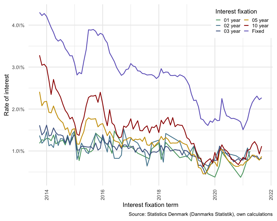
Figure 4.1: Danish interest rates
4.1.5 Density plots using ggplot2
ggplot2 offers a wide range of automatic image processing options. Including density plots.
density_plot_interest_rates <- ggplot() +
        geom_density(data = DK_yield_curves_rates,
                     mapping = aes(x = Value,
                            group = Interest_Fixation,
                            colour = Interest_Fixation)) +
    theme_extra +
    legend_top_right_inside +
    guides(col = guide_legend(nrow = 3,
                              byrow = FALSE,
                              title = "Interest fixation"))
density_plot_interest_rates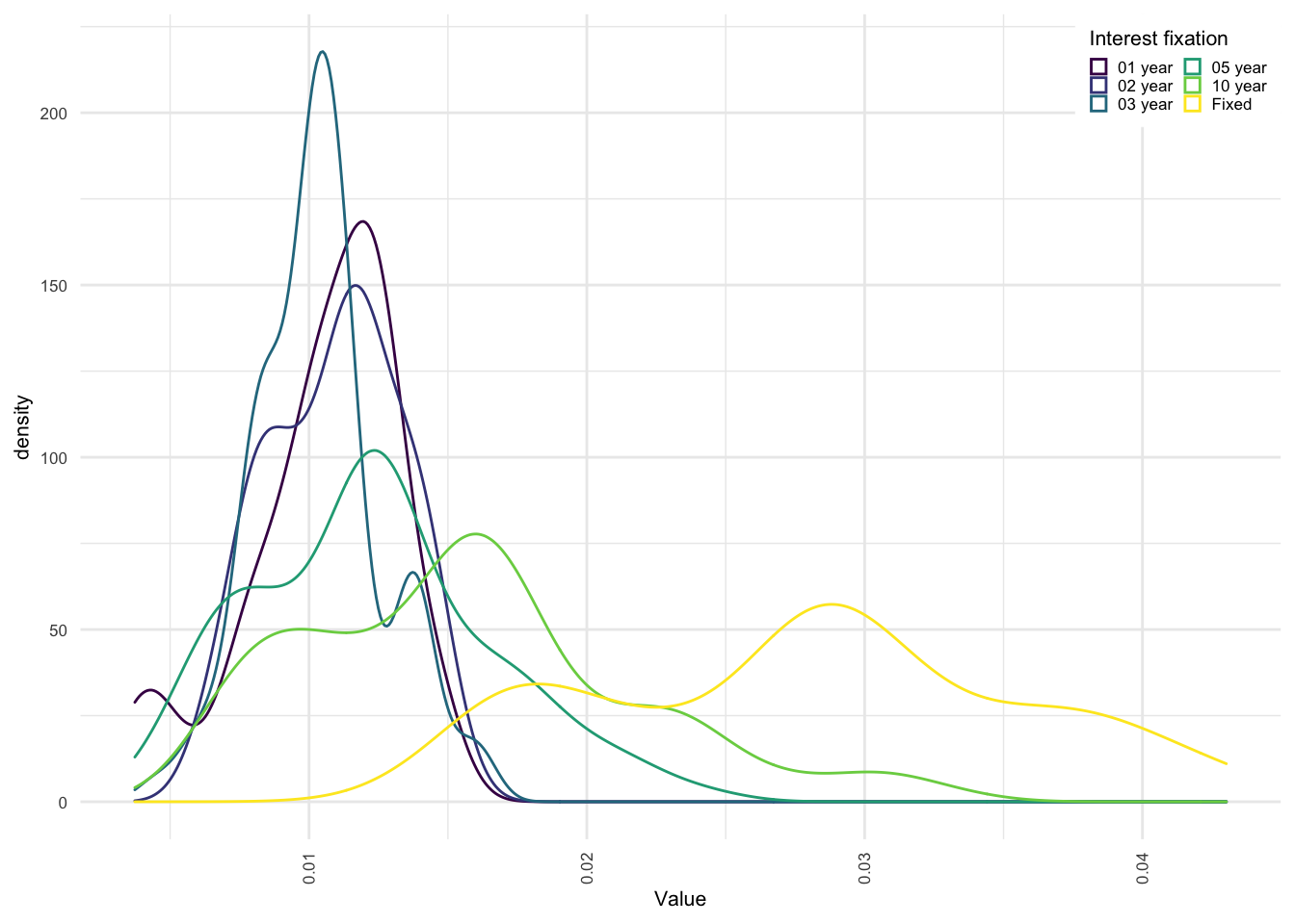
And the ability to automatically create a tiled “faceted” plot of underlying groupings.
density_plot_interest_rates <- ggplot() +
        geom_density(data = DK_yield_curves_rates,
                     mapping = aes(x = Value,
                            group = Interest_Fixation,
                            colour = Interest_Fixation)) +
    facet_wrap(~Interest_Fixation) +
    theme_extra +
    legend_top_right_inside +
    guides(col = guide_legend(nrow = 3,
                              byrow = FALSE,
                              title = "Interest fixation"))
density_plot_interest_rates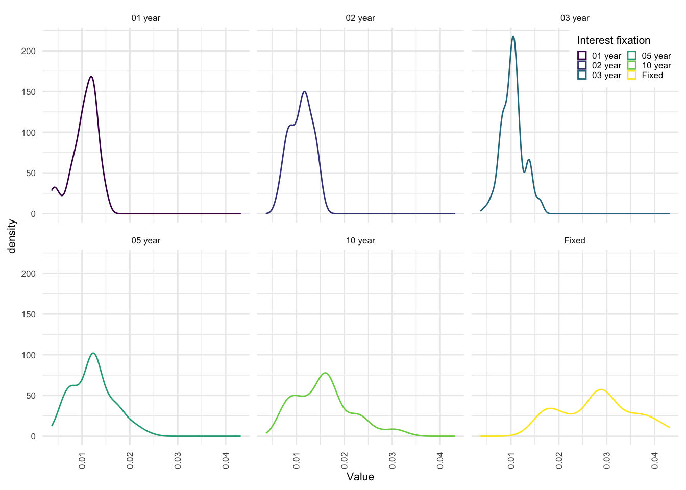
With minor modifications to the aes (aesthetics) properties, you can automatically change all plots to be filled in for these density plots. The Fill aesthetic is not available for all geom’s, so you will need to investigate the options for the ones that you are interested in.
You can see that I have also modified the number of rows in the legend to 6, to keep the legend narrower - since it overlaps the data in the top right corner. Additional legend options can be seen here. The identical legend settings and titles for col and fill prevent duplicate legends from being created. you can test this out by modifying one of the title texts.
The two options theme_extra, and legend_top_right_inside, are created above in the additional charting options section, and illustrate one way to keep your plotting code a little cleaner.
density_plot_interest_rates <- ggplot() +
        geom_density(data = DK_yield_curves_rates,
                     mapping = aes(x = Value,
                            group = Interest_Fixation,
                            colour = Interest_Fixation,
                            fill = Interest_Fixation)) +
    facet_wrap(~Interest_Fixation) +
    theme_extra +
    legend_top_right_inside +
    guides(col = guide_legend(nrow = 6,
                              byrow = FALSE,
                              title = "Interest fixation"),
           fill = guide_legend(nrow = 6,
                              byrow = FALSE,
                              title = "Interest fixation"))
density_plot_interest_rates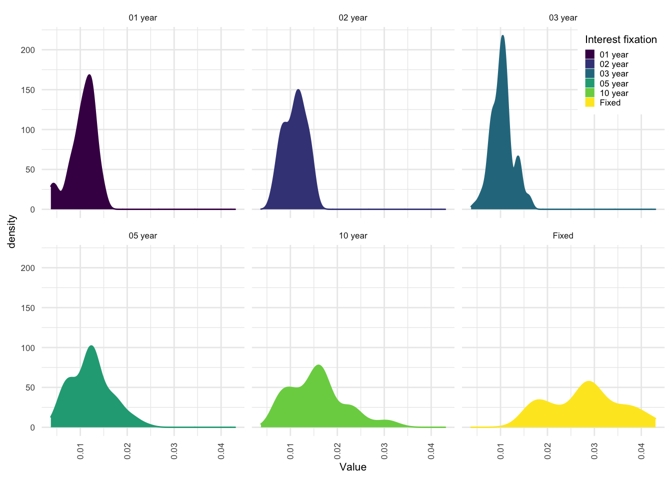
4.2 Example table
The kableExtra package provides some exceptionally simple quickformatting options for both html and PDF table generation. (Link to explainer page here)
The above sourced interest rate data can be quickly laid out in a table as follows:
pre_created_table <- DK_yield_curves_rates %>%
          arrange(Interest_Fixation) %>%
          spread(key = Interest_Fixation, value = Value)

pre_created_table %>%
  kbl(caption = "Table of interest rates over time") %>%
kable_styling(bootstrap_options = c("striped", "hover"))| Date | 01 year | 02 year | 03 year | 05 year | 10 year | Fixed |
|---|---|---|---|---|---|---|
| 2013-10-01 | 0.01183 | 0.01369 | 0.01613 | 0.02411 | 0.03282 | 0.04302 |
| 2013-11-01 | 0.01268 | 0.01185 | 0.01383 | 0.02078 | 0.03044 | 0.04229 |
| 2013-12-01 | 0.01252 | 0.01243 | 0.01448 | 0.02172 | 0.03067 | 0.04276 |
| 2014-01-01 | 0.01301 | 0.01459 | 0.01615 | 0.02183 | 0.02997 | 0.04208 |
| 2014-02-01 | 0.01294 | 0.01124 | 0.01357 | 0.01921 | 0.02680 | 0.04069 |
| 2014-03-01 | 0.01245 | 0.01155 | 0.01378 | 0.01909 | 0.02347 | 0.03945 |
| 2014-04-01 | 0.01380 | 0.01083 | 0.01550 | 0.02072 | 0.02705 | 0.03826 |
| 2014-05-01 | 0.01171 | 0.01405 | 0.01441 | 0.01918 | 0.02486 | 0.03681 |
| 2014-06-01 | 0.01209 | 0.01131 | 0.01382 | 0.01788 | 0.02397 | 0.03619 |
| 2014-07-01 | 0.01236 | 0.01295 | 0.01383 | 0.01723 | 0.02286 | 0.03656 |
| 2014-08-01 | 0.01256 | 0.01288 | 0.01362 | 0.01673 | 0.02114 | 0.03589 |
| 2014-09-01 | 0.01145 | 0.01181 | 0.01197 | 0.01510 | 0.01968 | 0.03442 |
| 2014-10-01 | 0.01309 | 0.01376 | 0.01334 | 0.01555 | 0.01891 | 0.03366 |
| 2014-11-01 | 0.01189 | 0.01186 | 0.01144 | 0.01368 | 0.01763 | 0.03269 |
| 2014-12-01 | 0.01272 | 0.01406 | 0.01318 | 0.01514 | 0.01804 | 0.03269 |
| 2015-01-01 | 0.01465 | 0.01474 | 0.01387 | 0.01532 | 0.01654 | 0.03083 |
| 2015-02-01 | 0.00796 | 0.01023 | 0.01168 | 0.01399 | 0.02812 | |
| 2015-03-01 | 0.00772 | 0.01024 | 0.01161 | 0.01373 | 0.02872 | |
| 2015-04-01 | 0.01061 | 0.01187 | 0.01110 | 0.01328 | 0.01633 | 0.02842 |
| 2015-05-01 | 0.01112 | 0.01465 | 0.01794 | 0.03145 | ||
| 2015-06-01 | 0.01061 | 0.00975 | 0.01099 | 0.01728 | 0.02083 | 0.03419 |
| 2015-07-01 | 0.00974 | 0.00938 | 0.01092 | 0.01789 | 0.02276 | 0.03888 |
| 2015-08-01 | 0.00983 | 0.01130 | 0.01105 | 0.01758 | 0.02313 | 0.03881 |
| 2015-09-01 | 0.01035 | 0.01043 | 0.01762 | 0.02309 | 0.03896 | |
| 2015-10-01 | 0.01427 | 0.01412 | 0.01193 | 0.01770 | 0.02328 | 0.03854 |
| 2015-11-01 | 0.01021 | 0.01576 | 0.02160 | 0.03752 | ||
| 2015-12-01 | 0.01188 | 0.01065 | 0.01632 | 0.02399 | 0.03803 | |
| 2016-01-01 | 0.01271 | 0.01328 | 0.01388 | 0.01653 | 0.02127 | 0.03778 |
| 2016-02-01 | 0.01200 | 0.01513 | 0.01803 | 0.03652 | ||
| 2016-03-01 | 0.00975 | 0.01159 | 0.01364 | 0.01602 | 0.03576 | |
| 2016-04-01 | 0.01084 | 0.01364 | 0.01246 | 0.01468 | 0.01983 | 0.03336 |
| 2016-05-01 | 0.00946 | 0.01117 | 0.01373 | 0.01669 | 0.03237 | |
| 2016-06-01 | 0.01477 | 0.00825 | 0.01105 | 0.01246 | 0.01613 | 0.03131 |
| 2016-07-01 | 0.01022 | 0.01225 | 0.01406 | 0.02989 | ||
| 2016-08-01 | 0.00824 | 0.01149 | 0.01207 | 0.01313 | 0.02893 | |
| 2016-09-01 | 0.00901 | 0.01058 | 0.01087 | 0.01335 | 0.02803 | |
| 2016-10-01 | 0.01101 | 0.01521 | 0.01145 | 0.01261 | 0.01594 | 0.02842 |
| 2016-11-01 | 0.01142 | 0.01265 | 0.01564 | 0.02941 | ||
| 2016-12-01 | 0.01108 | 0.01058 | 0.01309 | 0.01623 | 0.02955 | |
| 2017-01-01 | 0.01115 | 0.01296 | 0.01087 | 0.01322 | 0.01767 | 0.03084 |
| 2017-02-01 | 0.01114 | 0.01247 | 0.01522 | 0.03025 | ||
| 2017-03-01 | 0.00970 | 0.01283 | 0.03009 | |||
| 2017-04-01 | 0.00948 | 0.01188 | 0.01063 | 0.01269 | 0.01721 | 0.02911 |
| 2017-05-01 | 0.01074 | 0.01288 | 0.01486 | 0.02903 | ||
| 2017-06-01 | 0.00983 | 0.00978 | 0.01229 | 0.01481 | 0.02847 | |
| 2017-07-01 | 0.00979 | 0.01045 | 0.01330 | 0.01555 | 0.02839 | |
| 2017-08-01 | 0.00642 | 0.00992 | 0.01147 | 0.01599 | 0.02811 | |
| 2017-09-01 | 0.00813 | 0.00827 | 0.00896 | 0.01133 | 0.01430 | 0.02817 |
| 2017-10-01 | 0.01051 | 0.01198 | 0.00972 | 0.01207 | 0.01572 | 0.02818 |
| 2017-11-01 | 0.00980 | 0.01102 | 0.01558 | 0.02786 | ||
| 2017-12-01 | 0.00969 | 0.01168 | 0.01617 | 0.02727 | ||
| 2018-01-01 | 0.01184 | 0.01259 | 0.01004 | 0.01222 | 0.01440 | 0.02779 |
| 2018-02-01 | 0.00797 | 0.01133 | 0.01348 | 0.01733 | 0.02962 | |
| 2018-03-01 | 0.00735 | 0.01009 | 0.01266 | 0.01648 | 0.02858 | |
| 2018-04-01 | 0.01203 | 0.01417 | 0.01113 | 0.01321 | 0.01740 | 0.02882 |
| 2018-05-01 | 0.01089 | 0.01277 | 0.01802 | 0.02877 | ||
| 2018-06-01 | 0.00999 | 0.01184 | 0.01618 | 0.02801 | ||
| 2018-07-01 | 0.01016 | 0.01191 | 0.01795 | 0.02798 | ||
| 2018-08-01 | 0.01034 | 0.01189 | 0.01579 | 0.02805 | ||
| 2018-09-01 | 0.01021 | 0.01193 | 0.01631 | 0.02770 | ||
| 2018-10-01 | 0.00840 | 0.01218 | 0.01017 | 0.01249 | 0.01615 | 0.02816 |
| 2018-11-01 | 0.01051 | 0.00903 | 0.01195 | 0.01611 | 0.02793 | |
| 2018-12-01 | 0.01016 | 0.01169 | 0.01498 | 0.02760 | ||
| 2019-01-01 | 0.00882 | 0.00858 | 0.01002 | 0.01149 | 0.01319 | 0.02674 |
| 2019-02-01 | 0.00948 | 0.01021 | 0.01274 | 0.02565 | ||
| 2019-03-01 | 0.00763 | 0.00887 | 0.00901 | 0.01166 | 0.02359 | |
| 2019-04-01 | 0.01109 | 0.01114 | 0.00881 | 0.00922 | 0.01182 | 0.02202 |
| 2019-05-01 | 0.00853 | 0.00862 | 0.00998 | 0.02212 | ||
| 2019-06-01 | 0.00780 | 0.00655 | 0.00608 | 0.00831 | 0.02053 | |
| 2019-07-01 | 0.00663 | 0.00590 | 0.00828 | 0.01769 | ||
| 2019-08-01 | 0.00582 | 0.00453 | 0.00626 | 0.01744 | ||
| 2019-09-01 | 0.00448 | 0.00460 | 0.00728 | 0.01660 | ||
| 2019-10-01 | 0.00459 | 0.00643 | 0.00576 | 0.00545 | 0.00774 | 0.01609 |
| 2019-11-01 | 0.00723 | 0.00653 | 0.00817 | 0.01716 | ||
| 2019-12-01 | 0.00704 | 0.00793 | 0.00746 | 0.00723 | 0.01684 | |
| 2020-01-01 | 0.00378 | 0.00822 | 0.00772 | 0.00734 | 0.00966 | 0.01772 |
| 2020-02-01 | 0.00786 | 0.00633 | 0.00777 | 0.01723 | ||
| 2020-03-01 | 0.00655 | 0.01075 | 0.01116 | 0.01016 | 0.01004 | 0.01729 |
| 2020-04-01 | 0.00969 | 0.00971 | 0.01035 | 0.01038 | 0.01147 | 0.02249 |
| 2020-05-01 | 0.01019 | 0.00940 | 0.01047 | 0.01994 | ||
| 2020-06-01 | 0.00927 | 0.00829 | 0.01004 | 0.01839 | ||
| 2020-07-01 | 0.00879 | 0.00754 | 0.00941 | 0.01818 | ||
| 2020-08-01 | 0.00838 | 0.00716 | 0.00801 | 0.01774 | ||
| 2020-09-01 | 0.00743 | 0.00658 | 0.00786 | 0.01778 | ||
| 2020-10-01 | 0.00888 | 0.00778 | 0.00633 | 0.00726 | 0.01758 | |
| 2020-11-01 | 0.00818 | 0.00635 | 0.00675 | 0.01732 | ||
| 2020-12-01 | 0.00373 | 0.00762 | 0.00671 | 0.01690 | ||
| 2021-01-01 | 0.00487 | 0.00779 | 0.00823 | 0.00662 | 0.00846 | 0.01507 |
| 2021-02-01 | 0.00835 | 0.00742 | 0.00796 | 0.01630 | ||
| 2021-03-01 | 0.01072 | 0.00775 | 0.00763 | 0.01020 | 0.01752 | |
| 2021-04-01 | 0.00996 | 0.00834 | 0.00822 | 0.00821 | 0.01038 | 0.02004 |
| 2021-05-01 | 0.00891 | 0.00904 | 0.01161 | 0.02153 | ||
| 2021-06-01 | 0.00858 | 0.00895 | 0.01223 | 0.02243 | ||
| 2021-07-01 | 0.00882 | 0.00835 | 0.01134 | 0.02308 | ||
| 2021-08-01 | 0.00796 | 0.00782 | 0.00929 | 0.02223 | ||
| 2021-09-01 | 0.00829 | 0.00871 | 0.01115 | 0.02268 |
4.3 Interactive html plots with Plotly
A scatter plot with labels on all points can be easily created (some axis limits for the data were necessary below). I also wanted uniform dot sizes and so simply used Value / Value which returns 1 for all dot sizes.
library(plotly)

a <- as.numeric(min(DK_yield_curves_rates$Date)) * 24 * 60 * 60 * 1000
b <- as.numeric(max(DK_yield_curves_rates$Date)) * 24 * 60 * 60 * 1000

fig <- plot_ly(DK_yield_curves_rates %>%
    filter, x = ~Date, y = ~Value,
  # Hover text:
  text = ~paste("Interest rate: ", Value, '%<br>Fixation:', Interest_Fixation),
  mode = "markers",
  color = ~Value, size = ~Value/Value
) %>%
  layout(xaxis = list(range = c(a, b)))

fig
Modifying this plot to return lines, we just need to arrange the data in the correct order to ensure that the lines traced follow the correct pattern.
library(plotly)

a <- as.numeric(min(DK_yield_curves_rates$Date)) * 24 * 60 * 60 * 1000
b <- as.numeric(max(DK_yield_curves_rates$Date)) * 24 * 60 * 60 * 1000

fig <- plot_ly(DK_yield_curves_rates %>%
    arrange(Date),
    x = ~Date,
    y = ~Value,
    color = ~Interest_Fixation,
  # Hover text:
  text = ~paste("Interest rate: ", Value, '%<br>Fixation:', Interest_Fixation),
  mode = 'lines'
) %>%
  layout(xaxis = list(range = c(a, b)))

fig